My Contribution Overview
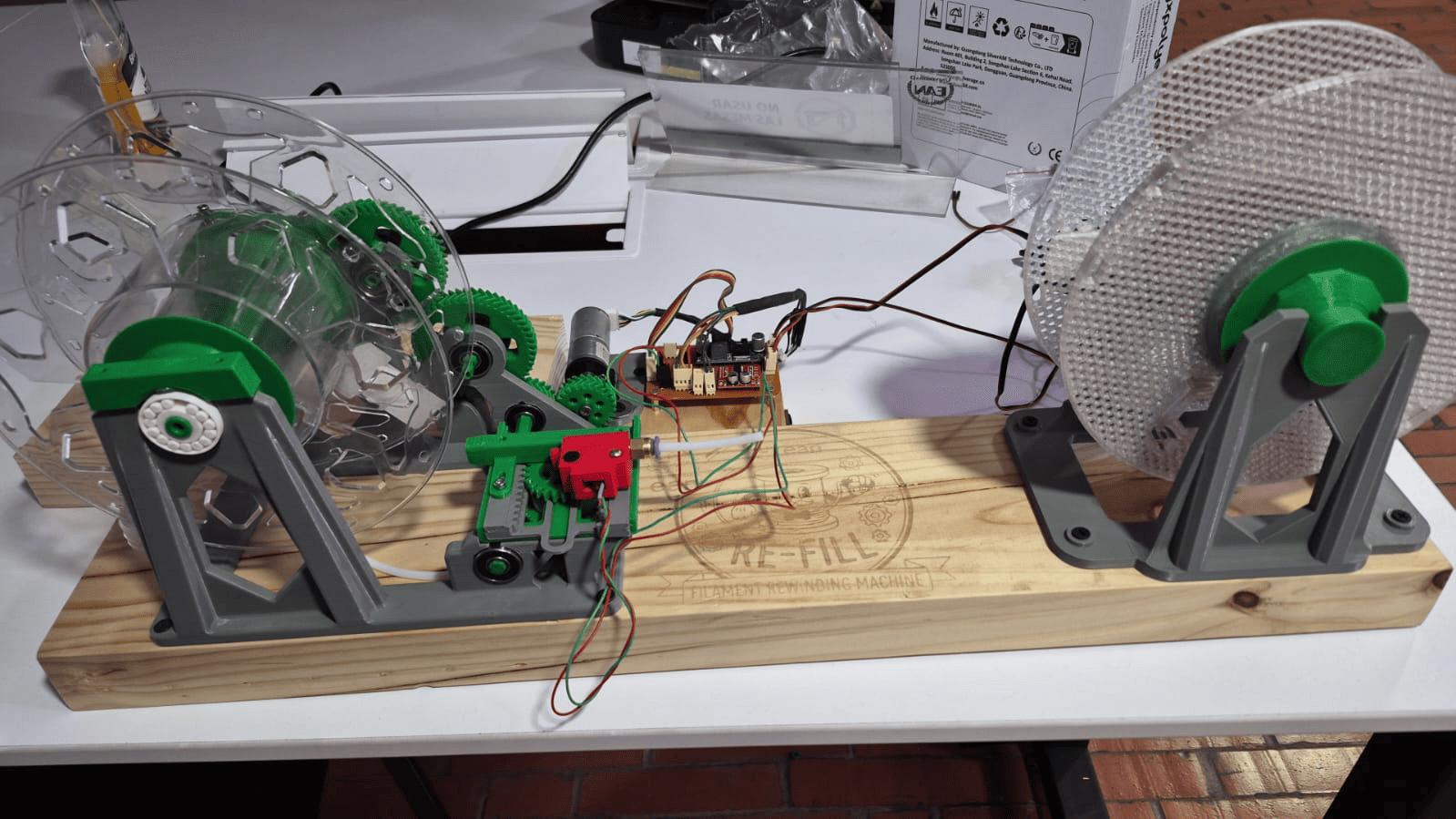
During the Mechanical Design and Machine Design week, our team developed ReFill, an automated filament rewinding machine capable of transferring filament from one spool to another in a controlled and reliable way.
While the project was developed collaboratively, my primary responsibility was the design and implementation of the electronic and embedded control system that enabled machine automation.
My Responsibilities
- Electronic schematic design
- PCB design and routing
- Generation of Gerber files for fabrication
- ESP32 firmware development
- Motor control implementation
- Hall-effect encoder integration
- OLED display interface development
- Hardware and software integration
- System testing and debugging
Learning Objectives
- Develop a complete embedded control system for a machine
- Design and fabricate a custom PCB
- Integrate sensors, actuators, and user interfaces
- Implement a state-machine-based control architecture
- Validate the interaction between hardware and software
- Collaborate effectively within a multidisciplinary team
Personal Development Status
Progress of the tasks assigned to me during the project.
Complete schematic design for the machine control system.
Routing, verification, and generation of fabrication files.
Development of machine control logic using ESP32.
Pulse counting and feedback system implementation.
Integration of electronics with the mechanical assembly.
Validation of motor control, sensors, and overall system behavior.
Project Overview & My Contribution
During the Mechanical Design and Machine Design week, our team developed ReFill, an automated filament rewinding machine designed to transfer filament from one spool to another in a controlled and efficient way.
The machine combines mechanical design, electronic control, and embedded programming to automate the rewinding process while improving filament organization and reducing material waste.
The complete development process, including the mechanical system, fabrication, assembly, testing, and team collaboration, is documented in the Group Assignment page.
My main contribution focused on the electronics and embedded control system. I was responsible for designing the electronic schematic, developing the custom PCB, generating fabrication files, programming the ESP32 firmware, integrating encoder feedback, and validating the interaction between hardware and software.
ReFill – Automated Filament Rewinding Machine
My Responsibilities
⚡ Electronics Design
Schematic development, PCB routing, and fabrication file generation.
💻 Firmware Development
ESP32 programming, motor control, encoder reading, and system logic.
🔗 System Integration
Integration of sensors, motor driver, OLED display, and PCB hardware.
🧪 Testing & Debugging
Validation of electronics, troubleshooting, and performance testing.
Electronic Design
My primary contribution to the ReFill project was the development of the electronic control system. The objective was to create a custom platform capable of controlling the motor, reading sensor feedback, interacting with the user, and coordinating the machine operation through an ESP32-based embedded system.
The electronics architecture was designed around a XIAO ESP32-C3 microcontroller, which communicates with the user interface, controls the motor driver, monitors the filament encoder, and executes the machine control logic.
Component Selection and System Integration
The design was developed around commercially available modules in order to accelerate prototyping while maintaining flexibility for future custom board revisions.
| Module | Purpose | Design Rationale |
|---|---|---|
| XIAO ESP32-C3 | Main Controller | Compact form factor, integrated WiFi/Bluetooth, low power consumption and sufficient GPIO availability. |
| SSD1306 OLED | User Interface | Provides real-time feedback while requiring only two communication lines through I²C. |
| Rotary Encoder | User Input | Allows intuitive navigation and parameter adjustment without requiring multiple buttons. |
| L298N Mini | Motor Driver | Enables bidirectional motor control and PWM speed regulation. |
| Hall Encoder | Position Feedback | Provides rotational information required to monitor spool turns. |
| LM2596 | Power Regulation | Generates a stable 5V rail from the machine power supply. |
Electronic Design Architecture
One of my main responsibilities in the ReFill project was the development of the electronic control system responsible for coordinating all machine operations.
The objective was to create a compact and modular platform capable of controlling the rewinding motor, reading rotational feedback, interacting with the user through a graphical interface, and executing the logic required to automate the filament transfer process.
To achieve this, I designed a custom architecture centered around the XIAO ESP32-C3, selected because it provides sufficient processing power, integrated wireless connectivity, compact dimensions, and compatibility with the development tools already used throughout Fab Academy.
The controller communicates with all peripherals including the rotary encoder, Hall-effect sensor, OLED display, motor driver, and future cutting mechanism. This centralized architecture simplifies maintenance while allowing future scalability.
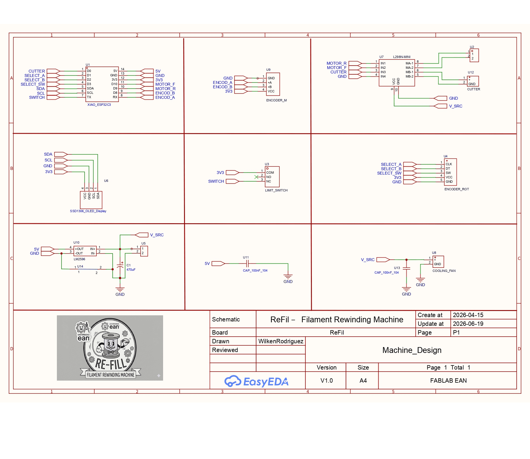
Complete electronic schematic developed for ReFill.
PCB Design Strategy
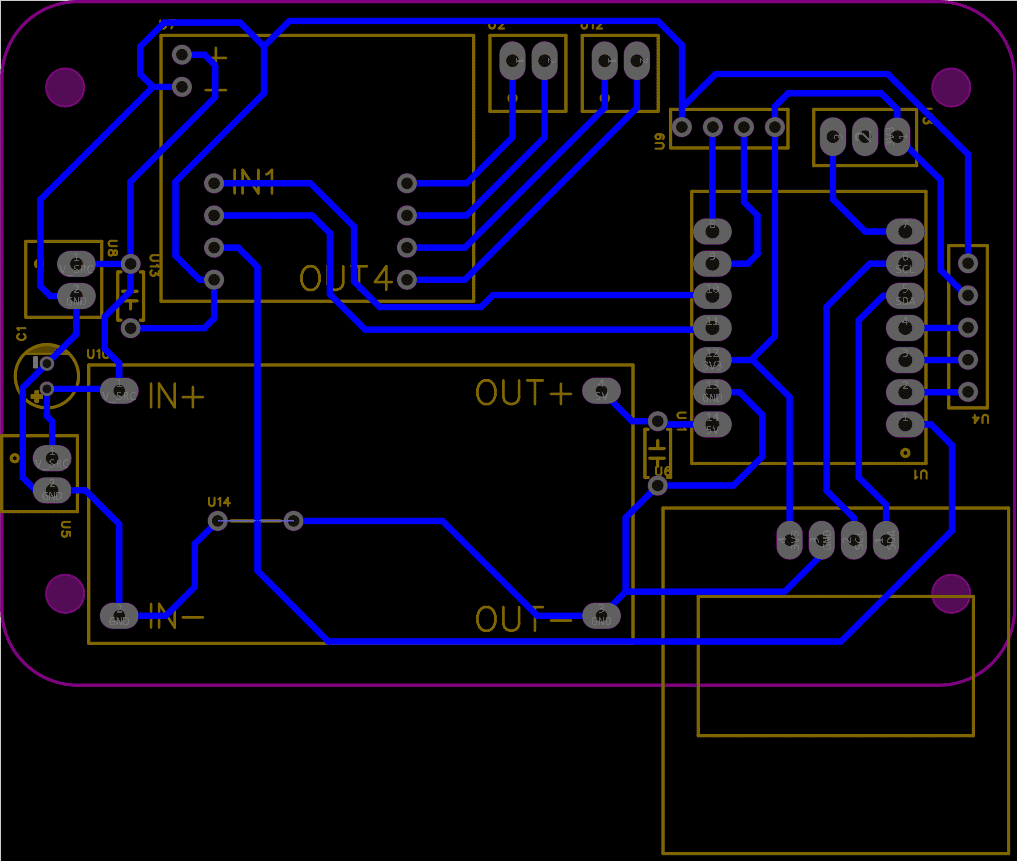
Final PCB routing performed on the bottom layer.
After validating the schematic, I developed a custom PCB to consolidate all electronic subsystems into a single board.
Because every selected component used through-hole connections or development-board headers, the PCB was intentionally designed using a single-layer routing approach.
All traces were routed on the bottom copper layer, reducing fabrication complexity and simplifying assembly inside the Fab Lab.
Special attention was given to connector accessibility, trace organization, and mechanical integration. The placement of each module was optimized to minimize routing conflicts while maintaining a clear separation between power distribution and signal lines.
This strategy resulted in a clean layout that can be easily assembled, repaired, and modified during future iterations.
3D Verification and Mechanical Integration
Before fabrication, I generated a complete 3D representation of the PCB assembly to validate the spatial arrangement of all components.
This step allowed verification of connector orientation, display positioning, module clearances, and accessibility during assembly.
The visualization also helped evaluate how the electronic system would integrate with the mechanical structure of the machine before investing time and materials into fabrication.
By identifying potential integration issues early in the design process, the 3D model reduced iteration cycles and increased confidence in the final implementation.
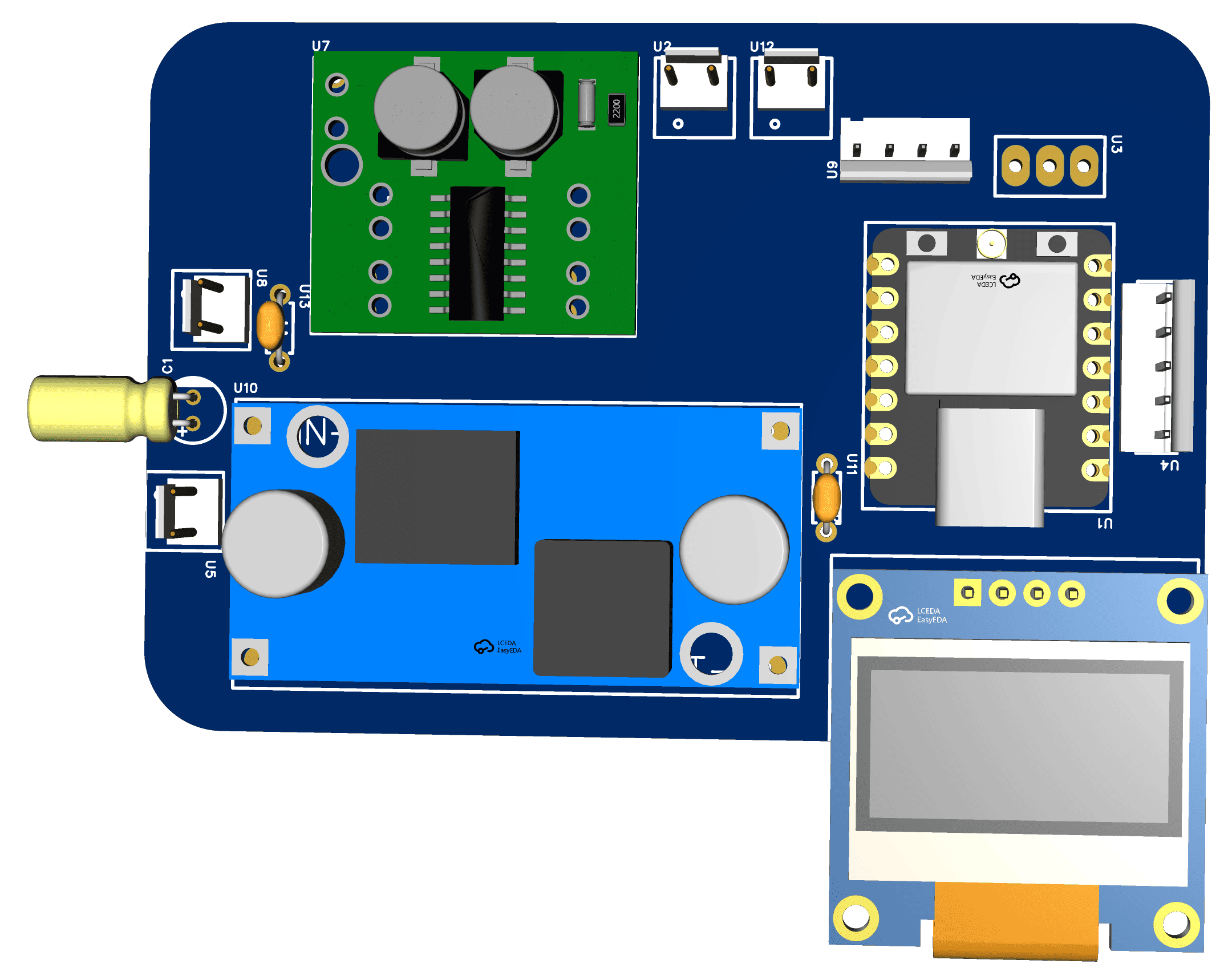
3D visualization of the complete PCB assembly.
PCB Assembly and Soldering Process
After completing the PCB design and fabrication process, the next stage consisted of assembling all electronic components onto the board. This step transformed the digital design into a functional control system ready for programming and integration with the machine.
The board was designed using through-hole components and development modules, which simplified assembly while maintaining flexibility for future modifications and troubleshooting. Each connector, module, and interface was carefully positioned according to the PCB layout developed during the design stage.
During soldering, particular attention was given to signal integrity, mechanical stability, and connector accessibility. Since the board would be integrated into a machine exposed to continuous movement, reliable electrical connections were essential for long-term operation.
Once assembly was completed, every connection was visually inspected and electrically verified before powering the system for the first time.
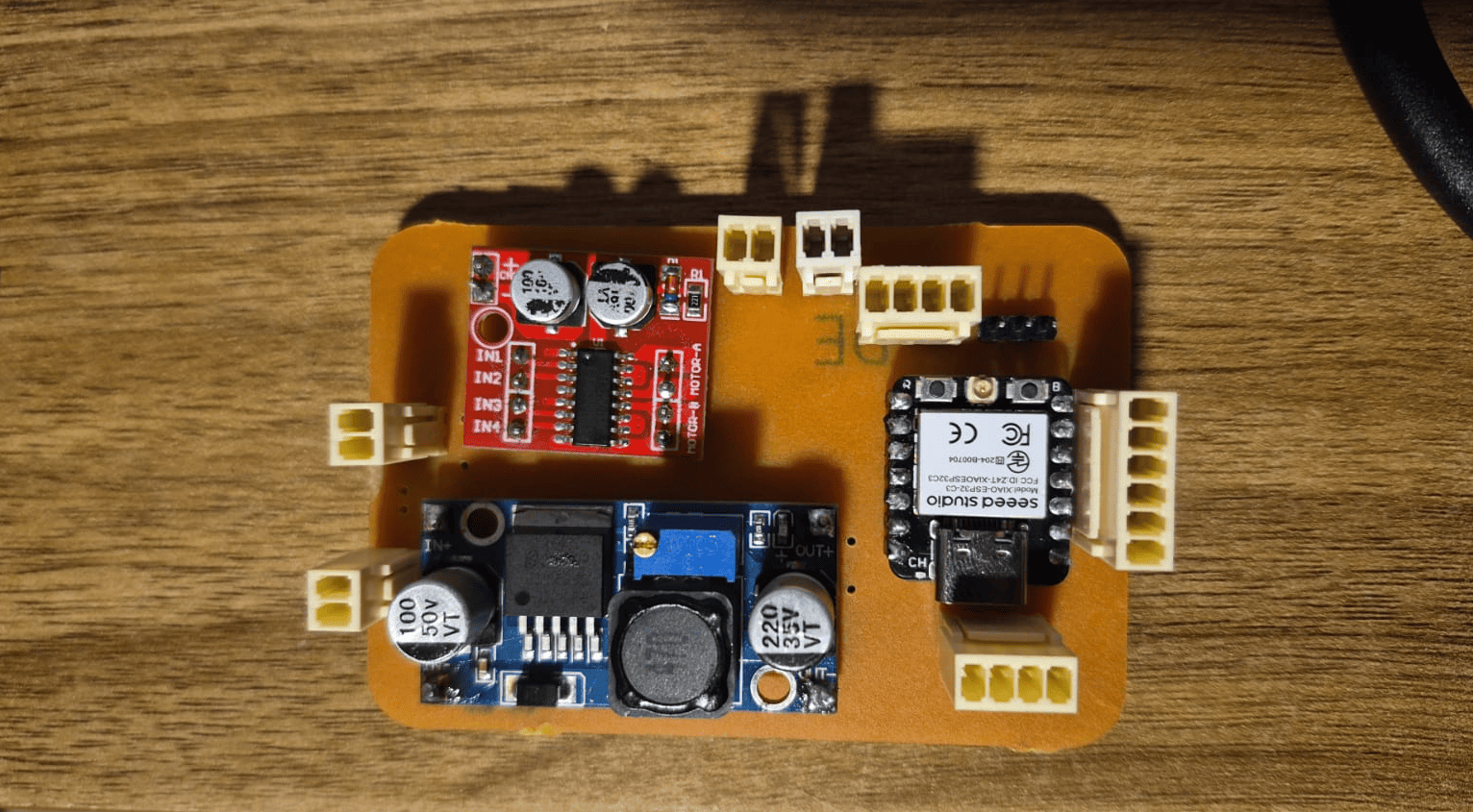
Fully assembled control board ready for testing and programming.
Inspection and Quality Verification
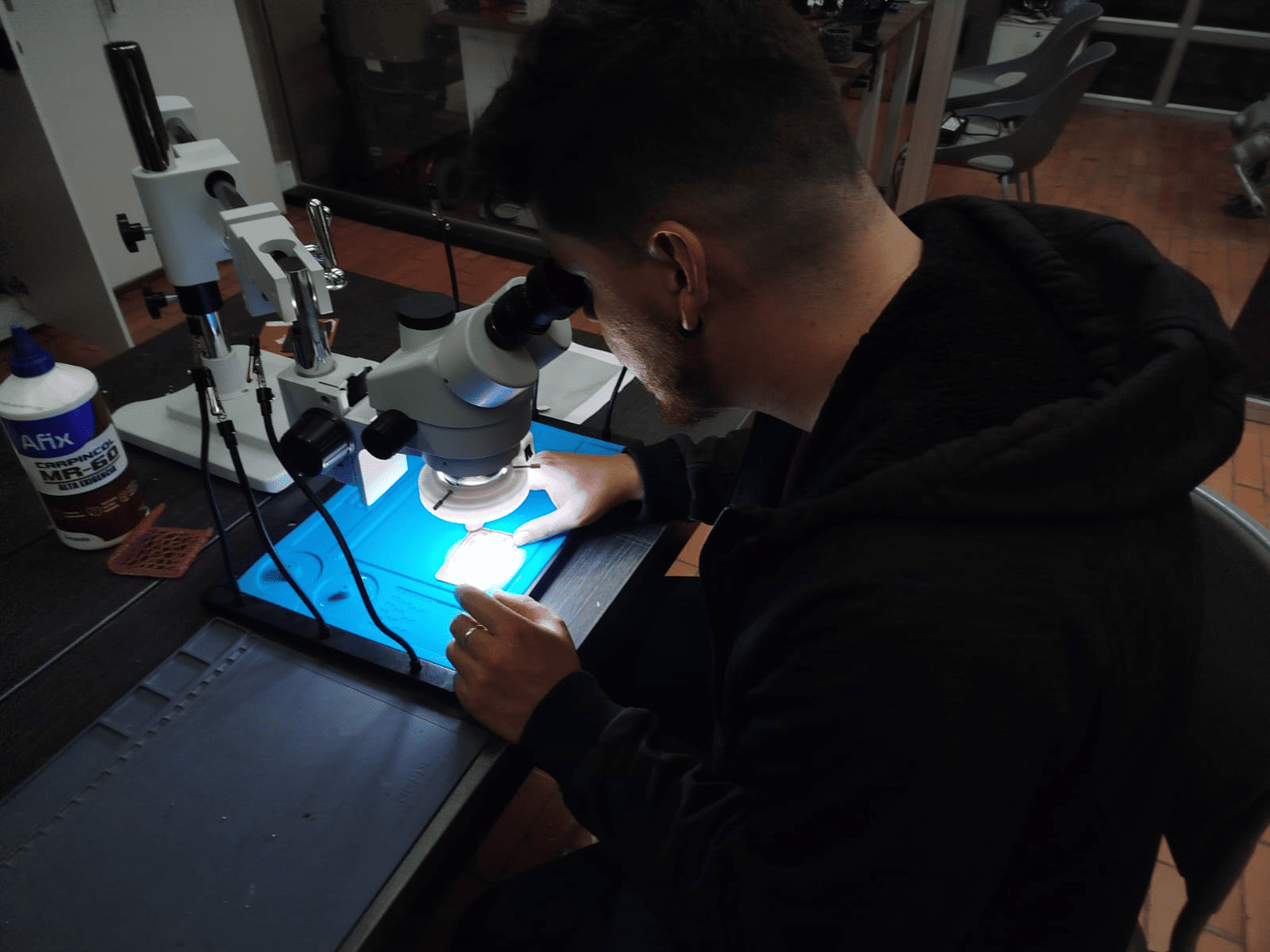
Verifying solder joints and electrical connections using a digital microscope.
Before integrating the electronics into the machine, the PCB was inspected under a digital microscope to verify solder quality and detect possible manufacturing defects.
This inspection process allowed the identification of potential cold joints, solder bridges, insufficient wetting, or alignment issues that could affect system reliability.
Using magnification tools significantly improves quality control, especially when working with densely packed traces and multiple interconnections between modules.
After confirming that all connections were correct, continuity tests and functional validation were performed to ensure the board was ready for firmware deployment and system integration.
Firmware Architecture
After completing the electronic design, I developed the embedded software responsible for coordinating all machine operations. The firmware was programmed using the Arduino framework running on the XIAO ESP32-C3 microcontroller.
The main objective was to create a reliable control system capable of managing user interaction, monitoring rotational feedback, controlling motor movement, and executing the rewinding sequence autonomously.
To simplify maintenance and improve scalability, the software was organized around a Finite State Machine (FSM). This approach separates machine behavior into clearly defined operational states, making the code easier to debug and expand.
Each state controls a specific phase of operation and defines the transitions required to move between them according to sensor inputs, user commands, and process completion conditions.
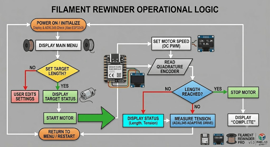
Finite State Machine used to coordinate machine behavior.
Machine Logic and Operational States
The firmware was structured around three operational states: IDLE, RUNNING, and CUTTING.
IDLE
Default state after power-up. The motor remains stopped while the user interacts with the menu, adjusts parameters, or starts a new rewinding cycle.
RUNNING
The motor rotates the spool while the Hall-effect encoder continuously measures rotational movement. The system compares the accumulated turns against the target value.
CUTTING
Once the programmed number of turns is reached, the motor stops and the cutting mechanism is activated before returning to the idle state.
enum Estado {
  IDLE,
  RUNNING,
  CUTTING
};
Hardware Initialization
During startup, the firmware initializes all hardware resources, including communication interfaces, GPIO pins, interrupts, PWM channels, and the OLED display.
This configuration stage ensures that every peripheral starts in a known state before entering the main control loop.
The motor driver, Hall sensor, user encoder, and display are all configured inside the setup routine, while the Hall sensor uses hardware interrupts to guarantee accurate pulse acquisition.
void setup() {

  Wire.begin(SDA_PIN, SCL_PIN);

  display.begin(
    SSD1306_SWITCHCAPVCC,
    0x3C
  );

  attachInterrupt(
    digitalPinToInterrupt(HALL_PIN),
    contarPulsos,
    RISING
  );

}
Rotational Feedback System
volatile long pulsos = 0;

void IRAM_ATTR contarPulsos() {
  pulsos++;
}
One of the most critical parts of the system is the rotational feedback mechanism.
A Hall-effect encoder generates pulses every time the spool rotates. These pulses are captured using an interrupt service routine, ensuring that no measurements are lost even while other tasks are executing.
The pulse count is continuously converted into spool turns, allowing the machine to determine when the desired rewinding objective has been reached.
Motor Control Strategy
The rewinding motor is controlled through an L298N driver using PWM signals generated by the ESP32.
PWM control allows speed regulation while maintaining a simple hardware architecture. The firmware can start, stop, and adjust motor behavior according to the active machine state.
During normal operation the motor rotates continuously until the target number of turns is reached or a safety condition is detected.
digitalWrite(MOTOR_R, LOW);
ledcWrite(
  pwmChannel,
  velocidad
);
User Interface and Navigation
void leerEncoderUI() {

  bool A = digitalRead(ENC_UI_A);

  if (A != lastUIA) {

    if (digitalRead(ENC_UI_B) != A)
      menuIndex++;
    else
      menuIndex--;

  }
}
User interaction is performed through a rotary encoder with an integrated push button.
Rotational movement allows navigation through menu options, while the push button executes the selected action.
This approach reduces the number of physical controls required while providing an intuitive interface for machine operation.
OLED Visualization System
Real-time feedback is presented through a 128x64 OLED display.
The interface continuously updates operational information such as the number of completed turns, target value, machine state, and available menu options.
This visualization system allows the user to monitor machine progress without requiring an external computer connection.
display.print("Vueltas: ");
display.println(vueltas);

display.print("Objetivo: ");
display.println(vueltasObjetivo);
Complete Firmware Implementation
After developing and validating each software module individually, the final firmware integrates user interaction, motor control, encoder feedback acquisition, state-machine logic, and OLED visualization into a single embedded application running on the XIAO ESP32-C3.
The program continuously monitors the Hall-effect encoder, processes user inputs through the rotary encoder, controls the rewinding motor using PWM, and updates the graphical interface in real time. The implementation follows the architecture described in the previous sections and serves as the central controller for the ReFill machine.
- Finite State Machine (FSM) architecture
- Interrupt-based Hall encoder acquisition
- PWM motor speed control
- Rotary encoder menu navigation
- OLED graphical user interface
- Automatic turn counting and process completion
- Limit switch safety monitoring
- Automatic cutter activation
View Complete Source Code
#include
#include
#include

// ================= PINOUT =================

// Encoder UI
#define ENC_UI_A D1
#define ENC_UI_B D2
#define ENC_UI_SW D3

// Encoder Hall (1 canal)
#define HALL_PIN D7

#define MOTOR_F D10
#define MOTOR_R D9

#define LIMIT_SWITCH D6
#define CUTTER D0
// ==========================================

// OLED
#define SCREEN_WIDTH 128
#define SCREEN_HEIGHT 64
Adafruit_SSD1306 display(SCREEN_WIDTH, SCREEN_HEIGHT, &Wire, -1);

// PWM
const int pwmChannel = 0;
const int pwmFreq = 5000;
const int pwmResolution = 8;
int velocidad = 180;

// Encoder UI
int menuIndex = 0;
bool lastUIA = LOW;

// Encoder Hall
volatile long pulsos = 0;

// CONFIGURACIÓN
int pulsosPorVuelta = 20;  // AJUSTAR según tu encoder
long vueltasObjetivo = 500;

// Estados
enum Estado {
  IDLE,
  RUNNING,
  CUTTING
};

Estado estado = IDLE;

// ================= INTERRUPCIÓN =================
void IRAM_ATTR contarPulsos() {
  pulsos++;
}

// ================= SETUP =================
void setup() {
  Wire.begin(SDA_PIN, SCL_PIN);
  display.begin(SSD1306_SWITCHCAPVCC, 0x3C);

  pinMode(ENC_UI_A, INPUT_PULLUP);
  pinMode(ENC_UI_B, INPUT_PULLUP);
  pinMode(ENC_UI_SW, INPUT_PULLUP);

  pinMode(HALL_PIN, INPUT_PULLUP);
  attachInterrupt(digitalPinToInterrupt(HALL_PIN), contarPulsos, RISING);

  pinMode(MOTOR_F, OUTPUT);
  pinMode(MOTOR_R, OUTPUT);

  pinMode(LIMIT_SWITCH, INPUT_PULLUP);
  pinMode(CUTTER, OUTPUT);

  ledcSetup(pwmChannel, pwmFreq, pwmResolution);
  ledcAttachPin(MOTOR_F, pwmChannel);

  pantallaInicio();
}

// ================= LOOP =================
void loop() {
  leerEncoderUI();
  manejarBoton();
  actualizarEstado();
  actualizarPantalla();
}

// ================= ENCODER UI =================
void leerEncoderUI() {
  bool A = digitalRead(ENC_UI_A);

  if (A != lastUIA) {
    if (digitalRead(ENC_UI_B) != A) menuIndex++;
    else menuIndex--;
  }

  lastUIA = A;

  if (menuIndex < 0) menuIndex = 0;
  if (menuIndex > 3) menuIndex = 3;
}

// ================= BOTÓN =================
void manejarBoton() {
  static bool last = HIGH;
  bool current = digitalRead(ENC_UI_SW);

  if (last == HIGH && current == LOW) {
    ejecutarOpcion();
    delay(200);
  }

  last = current;
}

// ================= ESTADOS =================
void actualizarEstado() {
  long vueltas = pulsos / pulsosPorVuelta;

  switch (estado) {

    case IDLE:
      detenerMotor();
      break;

    case RUNNING:
      if (digitalRead(LIMIT_SWITCH) == HIGH) {
        estado = IDLE;
        break;
      }

      digitalWrite(MOTOR_R, LOW);
      ledcWrite(pwmChannel, velocidad);

      if (vueltas >= vueltasObjetivo) {
        estado = CUTTING;
      }
      break;

    case CUTTING:
      detenerMotor();
      activarCutter();
      estado = IDLE;
      break;
  }
}

// ================= ACCIONES =================
void ejecutarOpcion() {
  switch (menuIndex) {

    case 0: // Start
      if (digitalRead(LIMIT_SWITCH) == LOW) {
        pulsos = 0;
        estado = RUNNING;
      }
      break;

    case 1: // Cut
      estado = CUTTING;
      break;

    case 2: // Reset
      pulsos = 0;
      break;

    case 3: // Ajustar objetivo
      vueltasObjetivo += 100;
      if (vueltasObjetivo > 5000) vueltasObjetivo = 100;
      break;
  }
}

void detenerMotor() {
  ledcWrite(pwmChannel, 0);
  digitalWrite(MOTOR_R, LOW);
}

void activarCutter() {
  digitalWrite(CUTTER, HIGH);
  delay(300);
  digitalWrite(CUTTER, LOW);
}

// ================= OLED =================
void actualizarPantalla() {
  long vueltas = pulsos / pulsosPorVuelta;

  display.clearDisplay();
  display.setTextSize(1);
  display.setCursor(0, 0);

  display.println("REBOBINADORA");

  display.print("Vueltas: ");
  display.println(vueltas);

  display.print("Objetivo: ");
  display.println(vueltasObjetivo);

  display.print("Estado: ");
  if (estado == IDLE) display.println("IDLE");
  if (estado == RUNNING) display.println("RUN");
  if (estado == CUTTING) display.println("CUT");

  display.println("");

  display.println(menuIndex == 0 ? "> Iniciar" : "  Iniciar");
  display.println(menuIndex == 1 ? "> Cortar" : "  Cortar");
  display.println(menuIndex == 2 ? "> Reset" : "  Reset");
  display.println(menuIndex == 3 ? "> Obj +" : "  Obj +");

  display.display();
}

void pantallaInicio() {
  display.clearDisplay();
  display.setTextSize(2);
  display.setCursor(10, 20);
  display.println("LISTO");
  display.display();
  delay(1000);
}
System Integration
Although my primary contribution focused on the electronic and embedded control system, the final validation of the project required the integration of these subsystems into the complete mechanical assembly developed by the team.
The custom control board was connected to the motor driver, Hall-effect encoder, user interface, limit switch, and power distribution system, allowing the machine to operate as a single coordinated platform.
Through this integration process, the firmware could interact directly with the mechanical transmission system, monitor spool rotation in real time, execute the programmed rewinding cycles, and provide feedback to the user through the OLED interface.
This stage was particularly valuable because it transformed the electronic prototype into a fully functional machine, validating both the hardware architecture and the software developed during the project.
The complete documentation of the mechanical design, fabrication, assembly process, transmission system, bearing arrangement, structural components, and final machine construction can be found in the Group Assignment documentation.
Final machine integrating the mechanical structure, electronics, and embedded control system.
Personal Reflection
This project represented one of the most complete and rewarding experiences of the Fab Academy so far because it brought together knowledge acquired throughout multiple previous assignments into a single functional machine.
From my perspective, the most valuable aspect was understanding how individual disciplines such as electronics design, PCB fabrication, embedded programming, and machine integration must work together to create a reliable system. While each of these topics had been explored separately during previous weeks, this project required combining them into a cohesive solution.
One of the biggest challenges was developing a control system capable of interacting with both the user and the mechanical components in real time. Designing the PCB, implementing the firmware architecture, managing encoder feedback, and validating the communication between all subsystems required multiple iterations and continuous testing.
The implementation of the finite state machine helped me better understand how software architecture influences the reliability and scalability of a machine. Likewise, working with interrupts, PWM control, sensor feedback, and user interfaces strengthened my confidence in embedded systems development.
Beyond the technical achievements, this project reinforced the importance of collaboration. The final machine was only possible because each team member contributed expertise from different areas, and seeing all subsystems come together into a working prototype was one of the most satisfying moments of the assignment.
Looking back, this project demonstrated how digital fabrication extends beyond producing individual parts. The real challenge lies in integrating mechanical, electronic, and software components into a complete system capable of solving a real-world problem. That integration process is the lesson I will carry forward into future projects.
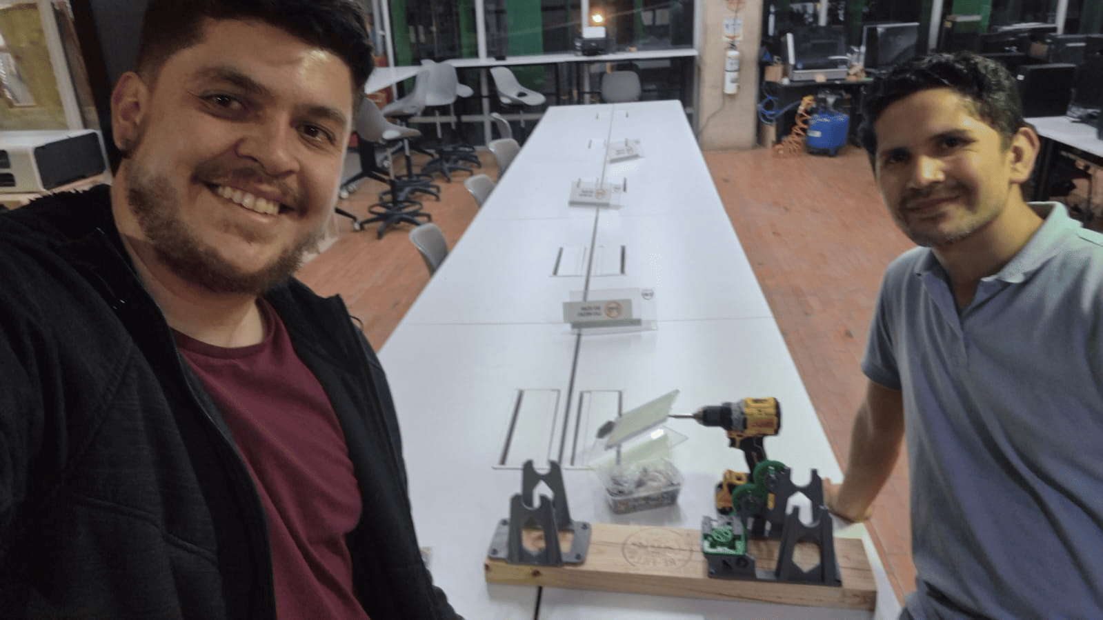
FABLAB EAN team building the final prototype of the ReFill filament rewinding machine.
Downloads & Resources
This section provides access to the design resources and downloadable files developed for the ReFill Machine. The repository includes the complete mechanical design, electronics, firmware, and supporting documentation required to reproduce the system.
🛠️ Project Resources
The project combines mechanical engineering, electronics, and embedded programming into a single machine. The repository includes every design file required for fabrication, assembly, and system operation.
- ✅ Mechanical CAD Models (3MF)
- ✅ PCB Design & Gerber Files
- ✅ Embedded Firmware Source Code
- ✅ Mechanical Assembly Resources
- ✅ Manufacturing Documentation
- ✅ Project Assets & Supporting Files
📁 Downloadable Files
To improve the loading performance of this documentation website, all project files have been moved to a shared Google Drive folder.
The repository contains the complete mechanical design, PCB fabrication files, embedded firmware, manufacturing resources, and supporting documentation developed for the ReFill Machine.
Future hardware revisions, firmware updates, and additional documentation may be added as the project continues to evolve.