Week 09

Individual Assignment Requirements

• Measure something: add a sensor to a microcontroller board that you have designed and read it.
• Demonstrate workflows used in sensing with input devices and a microcontroller.
• Document the design and fabrication process of the board used.
• Explain how the code works.
• Include problems encountered and how they were solved.
• Provide original design files and source code.
• Include a hero shot of the board.

Learning Outcomes

• Understand how analog and digital signals are read by a microcontroller.
• Work with multiple types of sensors and input devices.
• Visualize sensor data using displays and serial tools.
• Relate physical phenomena (temperature, motion, position) to digital readings.

System Overview – Input Devices Integration

This assignment focuses on exploring how a microcontroller can sense and interpret physical phenomena through different types of input devices. For this purpose, I worked with both analog and digital sensors connected to a custom PCB designed in a previous week, using a XIAO ESP32C3 as the main processing unit.

The objective was to measure and visualize different variables such as position, temperature, humidity, and motion. Each sensor was tested individually and the acquired data was displayed in real time using an SSD1306 OLED display, as well as analyzed through the Arduino IDE Serial Plotter to better understand signal behavior.

This approach allowed me to compare how analog signals (continuous values) and digital signals (discrete communication protocols) are handled by the microcontroller, and how each type of sensor requires a different strategy for reading and processing data.

All experiments were implemented on the same hardware platform, enabling a modular and efficient workflow for testing multiple input devices without modifying the base system.

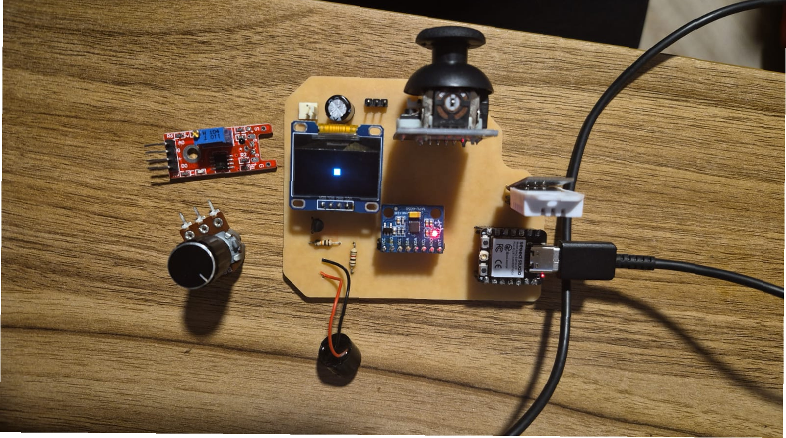
Complete system setup showing the custom PCB, XIAO ESP32C3, multiple input devices, and real-time visualization on the OLED display.

Experiment 1 – Potentiometer (Analog Input)

In this first experiment, I used a potentiometer as an analog input device to understand how continuous signals are read by the microcontroller. The potentiometer outputs a variable voltage depending on its position, which is converted into a digital value using the ADC (Analog-to-Digital Converter).

The XIAO ESP32C3 features a 12-bit ADC resolution, meaning the analog signal is mapped into a digital range from 0 to 4095. This allows a detailed and precise representation of the physical movement of the potentiometer.

The measured values were visualized in two ways: first, on an SSD1306 OLED display for real-time feedback, and second, using the Arduino IDE Serial Plotter, which allowed observing the continuous variation of the signal as the potentiometer was rotated.

This experiment demonstrates how analog inputs provide smooth transitions compared to digital signals, making them ideal for measuring variables such as position, light, or temperature.

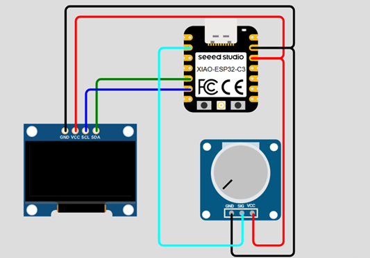
Potentiometer connected to analog input pin (Wokwi simulation).

Program Code

// ANALOG READING (0 - 4095)
// POTENTIOMETER TEST

#include <Wire.h>
#include <Adafruit_GFX.h>
#include <Adafruit_SSD1306.h>

// DISPLAY CONFIG
#define heigth 64 
#define width  128
#define rst   -1
Adafruit_SSD1306 oled(width, heigth, &Wire, rst);

// PIN
#define potentiometer D0  

void setup() {
  boardBegin();

  Serial.println("POTENTIOMETER - ANALOG INPUT TEST");

  oled.clearDisplay();
  oled.setTextSize(2);
  oled.println("POTENTIOMETER");
  oled.println("ANALOG INPUT");
  oled.display();

  delay(4000);
}

void loop() {

  int sensorReading = analogRead(potentiometer);

  oled.clearDisplay();
  oled.setTextSize(1);
  oled.setCursor(0, 0);

  oled.println("POTENTIOMETER DATA");
  oled.println("RANGE : (0 - 4095)\n");

  oled.print("POSITION_LEVEL: ");
  oled.println(sensorReading);

  Serial.print("POSITION_LEVEL:");
  Serial.println(sensorReading);

  oled.display();

  delay(100);
}

void boardBegin(){

  pinMode(potentiometer, INPUT);

  Serial.begin(115200);
  Wire.begin();

  if(!oled.begin(SSD1306_SWITCHCAPVCC, 0x3C)){
    Serial.println("Oled Display NOT Found...");
    for (;;);
  }

  oled.setTextColor(WHITE);
  oled.clearDisplay();
  oled.setTextSize(1);
  oled.setCursor(5, 5);
}
  

Code Explanation

• Libraries and Communication: The Wire.h library enables I2C communication, which is required for the OLED display. The Adafruit_GFX and Adafruit_SSD1306 libraries provide high-level functions to control graphics, text rendering, and display buffer management.
• Display Initialization: The OLED display is defined as an object with a resolution of 128x64 pixels. Inside the boardBegin() function, the display is initialized using oled.begin() with the I2C address 0x3C. If the display is not detected, the program stops execution using an infinite loop, which is useful for debugging hardware connections.
• Pin Configuration: The potentiometer is connected to pin D0, which is configured as an input using pinMode(). This pin is used by the ADC to measure the analog voltage.
• Analog-to-Digital Conversion (ADC): The function analogRead() converts the input voltage into a digital value. Since the ESP32C3 uses a 12-bit ADC, the output range is from 0 to 4095. This means small variations in voltage are translated into fine numerical changes, allowing precise detection of the potentiometer position.
• Main Loop Behavior: In the loop() function, the system continuously reads the analog value, updates the display, and sends the data through the serial port. This creates a real-time feedback system where any physical interaction with the potentiometer is immediately reflected in both outputs.
• OLED Display Rendering: Before printing new data, the display buffer is cleared using oled.clearDisplay(). Text properties such as size and cursor position are configured with setTextSize() and setCursor(). The data is written into a memory buffer and only becomes visible when oled.display() is executed. This buffered approach prevents flickering and ensures smooth updates.
• Serial Communication and Plotting: The sensor value is sent using Serial.print() and Serial.println(). This allows the Arduino IDE Serial Plotter to interpret the incoming data as a continuous signal. As a result, the potentiometer movement can be visualized as a real-time graph, making it easier to analyze signal stability, noise, and responsiveness.
• Timing Control: A delay of 100 ms is introduced to control the refresh rate. This prevents excessive data flooding in the Serial Plotter and ensures stable visualization on the OLED display without flickering or performance issues.

System in Operation

Experiment 2 – Analog Temperature Sensor

In this experiment, I used an analog temperature sensor to measure thermal variation. Unlike the previous case, this sensor represents temperature as a continuous voltage signal, which is read by the microcontroller using the ADC.

Since no calibrated reference in degrees Celsius was available, a relative measurement approach was implemented. The system was normalized using a percentage scale, where 0% corresponds to ambient temperature and 100% corresponds to the temperature of a soldering iron when the sensor is placed close to it.

The ESP32C3 reads the analog signal with a 12-bit resolution (0–4095), and then the map() function is used to convert this raw range into a normalized scale from 0 to 100%. This allows an intuitive interpretation of temperature variation even without an absolute reference.

As in the previous experiment, the processed data is displayed on the OLED screen and simultaneously sent to the Serial Plotter, enabling visualization of how the temperature changes dynamically when the sensor is exposed to different heat sources.

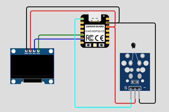
Analog temperature sensor connected to the microcontroller (Wokwi simulation).

Program Code

// ANALOG READING (0 - 4095)
// TEMPERATURE NORMALIZATION (0 - 100%)

#include <Wire.h>
#include <Adafruit_GFX.h>
#include <Adafruit_SSD1306.h>

// DISPLAY CONFIG
#define heigth 64 
#define width  128
#define rst   -1
Adafruit_SSD1306 oled(width,heigth,&Wire,rst);

// PIN
#define sensor D0  

void setup() {
  
  boardBegin();

  Serial.println("TEMPERATURE SENSOR TEST");

  oled.clearDisplay();
  oled.println("TEMP SENSOR TEST");
  oled.display();

  delay(2000);
}

void loop() {

  int sensorReading = analogRead(sensor);

  // Map raw ADC values to percentage scale
  sensorReading = map(sensorReading, 1000, 250, 0, 100);

  oled.clearDisplay();
  oled.setCursor(0, 10);

  oled.println("TEMP SENSOR DATA");
  oled.println("RANGE : (0 - 100%)\n");

  oled.print("TEMPERATURE_LEVEL: ");
  oled.print(sensorReading);
  oled.println("%");

  Serial.print("TEMPERATURE_LEVEL:");
  Serial.println(sensorReading);

  oled.display();

  delay(100);
}

void boardBegin(){

  pinMode(sensor, INPUT);

  Serial.begin(115200);
  Wire.begin();

  if(!oled.begin(SSD1306_SWITCHCAPVCC, 0x3C)){
    Serial.println("Oled Display NOT Found...");
    for (;;);
  }

  oled.setTextColor(WHITE);
  oled.clearDisplay();
  oled.setTextSize(1);
  oled.setCursor(5, 5);
}
  

Code Explanation

• Reuse of Previous Structure: This program follows the same structure as the potentiometer experiment, including OLED initialization, Serial communication, and continuous reading inside the loop(). These elements are reused to maintain a consistent workflow for data acquisition and visualization.
• Analog Temperature Reading: The temperature sensor outputs a voltage that varies according to thermal conditions. This signal is read using analogRead(), producing a 12-bit value between 0 and 4095, similar to the previous experiment.
• Experimental Calibration: Instead of using predefined values, two reference points were obtained experimentally: ambient temperature (~1000) and soldering iron temperature (~250). These values define the working range of the sensor in this setup.
• Normalization using map(): The key difference in this experiment is the use of the map() function. This function converts the raw ADC values into a percentage scale from 0 to 100. The mapping is inverted (1000 → 0%, 250 → 100%) due to the sensor's response when exposed to heat.
• Relative Measurement Approach: Since no absolute temperature reference (°C) is available, the system works with a normalized scale. This allows interpreting temperature variation in a meaningful way without requiring precise calibration.
• Data Visualization: The mapped value is displayed as a percentage on the OLED screen and sent to the Serial Plotter. This makes it possible to observe how temperature changes over time as the sensor moves between ambient conditions and the heat source.

System in Operation

Experiment 3 – Joystick Control (Analog Input)

In this experiment, a joystick module was used as a dual analog input device to control the position of a square displayed on the OLED screen. The joystick contains two potentiometers, one for each axis (X and Y), allowing two-dimensional movement.

A key challenge in this experiment was understanding that the joystick has a mechanical return to its center position. This means that the analog reading cannot be directly mapped to the position of the square. Instead, the readings must be interpreted as relative changes (movement direction), not absolute position.

Initially, it was assumed that the center value would be exactly 2048 (midpoint of a 12-bit ADC). However, experimental measurements showed that the real center values were different for each axis (X ≈ 2222, Y ≈ 2159). This caused unintended movement of the square even when the joystick was not being touched.

This issue was solved by calibrating the center values and introducing a threshold range. Only when the deviation exceeds this threshold, the position of the square is updated, allowing stable and controlled movement.

The system also demonstrates how basic geometric shapes can be drawn on the OLED display using graphic functions, enabling simple interactive interfaces.

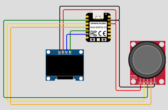
Joystick module connected as dual analog input (X and Y axes).

Program Code

#include <Adafruit_GFX.h>
#include <Adafruit_SSD1306.h>
#include <Wire.h>

// Pin definition
#define SDA D4
#define SCL D5
#define potY D1
#define potX D2

// Display configuration
#define height 64
#define width 128 
#define rst    -1

Adafruit_SSD1306 display(width, height, &Wire, rst);

// Process variables
int potValue = 0;
unsigned int posX = 64-5, posY = 32-5;

// Calibrated center values for joystick axes
int centro[2] = {2222, 2159};

void setup() {
  Serial.begin(115200);
  Wire.begin();

  if(!display.begin(SSD1306_SWITCHCAPVCC, 0X3C)){
    Serial.println("Oled Display NOT Found...");
    for(;;);
  }

  displayTxtConfig(2, 15, 0);
  display.clearDisplay();
  display.println("PongBALL");

  displayTxtConfig(2, 40, 30);
  display.println("GAME");

  display.display();

  Serial.println("SquarePoint Control");
  delay(3000);
}

void loop() {

  // Read joystick values
  int lectura[2];
  lectura[0] = analogRead(potX);
  lectura[1] = analogRead(potY);

  // Evaluate movement using threshold
  if(lectura[0] - centro[0] > 100){ posX += 1; }
  if(lectura[0] - centro[0] < -100){ posX -= 1; }

  if(lectura[1] - centro[1] > 100){ posY -= 1; }
  if(lectura[1] - centro[1] < -100){ posY += 1; }

  // Draw square at current position
  pintarCuadrado(posX, posY);

  // Screen wrapping logic
  if(posX > 127){ posX = 1; }
  if(posX < 1){ posX = 127; }

  if(posY > 63){ posY = 1; }
  if(posY < 1){ posY = 63; }

  // Serial output for debugging
  Serial.print("LecturaX:");
  Serial.print(lectura[0]);
  Serial.print("\t");

  Serial.print("LecturaY:");
  Serial.println(lectura[1]);
}

// Configure text properties
void displayTxtConfig(int size, int x, int y){
  display.setTextSize(size);
  display.setTextColor(WHITE);
  display.setCursor(x, y);
}

// Draw square on display
void pintarCuadrado(int x, int y){
  display.clearDisplay();
  display.fillRect(x, y, 10, 10, WHITE);
  display.display();
}
  

Code Explanation

• Reuse of Previous Concepts: The program builds on previous experiments by reusing OLED initialization, I2C communication, and analog input reading. However, this experiment introduces more advanced interaction logic and graphical rendering.
• Dual Analog Input (Joystick Axes): The joystick integrates two potentiometers, one for each axis (X and Y). These are read independently using analogRead(), producing two 12-bit values that represent the joystick position in two dimensions.
• ⚠️ Initial Design Error – Direct Mapping: At first, the position of the square on the screen was directly linked to the analog readings. This caused unstable and unintuitive behavior, since even small variations or noise in the signal resulted in large jumps in position. Additionally, due to the joystick's mechanical return to center, the square would always move back instead of staying in place.
• ⚠️ Center Value Assumption Error: It was initially assumed that the center value of the joystick would be exactly 2048 (midpoint of a 12-bit ADC). However, real measurements showed that each axis has a different center value (X ≈ 2222, Y ≈ 2159). This caused unintended movement even when the joystick was not being touched.
• Center Calibration Solution: To fix this, calibrated center values were stored in the array centro[2]. This allows the system to correctly interpret when the joystick is at rest.
• Relative Movement (Delta-Based Control): Instead of using absolute position, the program calculates the difference between the current reading and the calibrated center. If the difference exceeds a defined threshold, the position of the square is incremented or decremented. This creates a smooth and controllable interaction model.
• Threshold Filtering: A threshold of ±100 is applied to ignore small fluctuations and noise around the center position. This prevents jitter and improves control stability.
• Position State Variables: The variables posX and posY store the current position of the square. These are updated incrementally, meaning the system behaves more like velocity control rather than absolute positioning.
• Graphics Rendering – Adafruit GFX: The function fillRect(x, y, width, height, color) is used to draw a filled square on the OLED display. This demonstrates how geometric primitives can be used to create interactive graphical elements.
• Display Refresh Strategy: The display is cleared using clearDisplay() before drawing each frame. Then, display() updates the screen buffer. This creates a frame-by-frame rendering system similar to basic graphics engines.
• Screen Wrapping Logic: When the square reaches the edge of the display, its position is reset to the opposite side. This creates a continuous movement effect and avoids boundary locking.
• Modular Functions: Two helper functions are introduced:
  • displayTxtConfig(): Configures text size, color, and cursor position.
  • pintarCuadrado(): Handles drawing and updating the square on screen.
  This modular structure improves readability and code reuse.
• Serial Debugging: The raw values of both axes are sent through Serial communication. This allows real-time monitoring of joystick behavior and helps verify calibration and threshold performance.

System in Operation

This experiment highlights the importance of interpreting sensor data correctly, especially when dealing with input devices that include mechanical behavior, such as automatic centering.

Experiment 4 – DHT22 (Digital Temperature & Humidity Sensor)

In this experiment, a DHT22 sensor was used to measure ambient temperature and humidity. Unlike previous experiments, this is a digital sensor, meaning it does not output a continuous voltage signal, but instead communicates data through a digital protocol.

Analog sensors provide a voltage that must be interpreted using the ADC, resulting in values between 0 and 4095 (12-bit resolution). In contrast, digital sensors like the DHT22 internally process the signal and send already-calibrated data (temperature in °C and humidity in %) directly to the microcontroller.

To interface with this sensor, a dedicated library from Adafruit was used. This simplifies communication by handling the timing-sensitive protocol required by the DHT22, allowing the program to directly read temperature and humidity values.

The same visualization strategy from previous experiments was maintained: data is displayed on the OLED screen and simultaneously sent to the Serial Plotter, ensuring consistency in how sensor data is interpreted and analyzed.

⚠️ During testing, the sensor was accidentally connected in reverse, which caused permanent damage to the component. This highlighted the importance of hardware protection. A recommended solution is adding a protection diode in the VCC line to prevent reverse polarity from damaging external peripherals. However, the system was previously validated in simulation, confirming that the code and logic were correct.

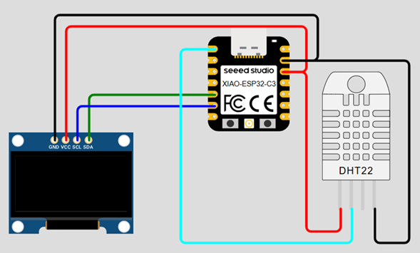
DHT22 digital sensor connected to the microcontroller.

Program Code

// LIBRARIES
#include <Wire.h>
#include <Adafruit_GFX.h>
#include <Adafruit_SSD1306.h>
#include "DHT.h"

// DISPLAY CONFIG
#define heigth 64 
#define width  128
#define rst   -1
Adafruit_SSD1306 oled(width,heigth,&Wire,rst);

// PIN DEFINITION
#define sensor D0  

// DHT CONFIG
#define DHTTYPE DHT22  
DHT sTemp(sensor, DHTTYPE);

void setup() {
  
  boardBegin();

  Serial.println("DHT SENSOR TEST");

  oled.clearDisplay();
  oled.println("DHT SENSOR TEST");
  oled.display();

  delay(2000);
}

void loop() {

  // Read humidity and temperature
  float h = sTemp.readHumidity();
  float t = sTemp.readTemperature();
  float f = sTemp.readTemperature(true);

  oled.clearDisplay();
  oled.setCursor(0, 10);

  oled.println("SENSOR DATA\n");

  oled.print("TEMP: ");
  oled.print(t);
  oled.println("C\n");

  oled.print("HUM: ");
  oled.print(h);
  oled.println("%");

  Serial.print("TEMP:");
  Serial.print(t);
  Serial.print("\t");

  Serial.print("HUM:");
  Serial.println(h);

  oled.display();

  delay(100);
}

void boardBegin(){

  Serial.begin(115200);
  Wire.begin();

  if(!oled.begin(SSD1306_SWITCHCAPVCC, 0x3C)){
    Serial.println("Oled Display NOT Found...");
    for (;;);
  }

  oled.setTextColor(WHITE);
  oled.clearDisplay();
  oled.setTextSize(1);
  oled.setCursor(5, 5);
}
  

Code Explanation

• Reuse of Previous Structure: The OLED display configuration and Serial communication follow the same structure used in previous experiments, ensuring consistency in data visualization.
• Digital Sensor Integration: Unlike analog sensors, the DHT22 communicates using a digital protocol. The DHT.h library abstracts this complexity, allowing simple function calls to retrieve sensor data.
• DHT Object Initialization: The sensor is initialized using: DHT sTemp(sensor, DHTTYPE); where the pin and sensor type are defined. This object handles all communication.
• Sensor Data Acquisition: The methods readHumidity() and readTemperature() are used to obtain calibrated values directly in physical units (°C and %). This is a key difference from analog sensors, where raw values must be interpreted.
• Built-in Data Processing: The sensor internally processes the signal and returns meaningful values, eliminating the need for ADC conversion or manual scaling.
• OLED and Serial Output: The measured temperature and humidity are displayed on the OLED screen and sent via Serial communication, maintaining the same visualization workflow used in previous experiments.
• ⚠️ Hardware Error – Reverse Connection: During testing, the sensor was connected incorrectly (reversed polarity), resulting in permanent damage.
• ⚠️ Protection Strategy: A diode can be added in series with the VCC line to prevent reverse current flow. This simple hardware protection can avoid damaging sensors and improve system reliability.

System in Operation

Experiment 5 – MPU6050 (6-Axis IMU)

In this experiment, an MPU6050 sensor was used, which is a 6-axis IMU (Inertial Measurement Unit). An IMU is a device that measures motion and orientation using a combination of sensors.

The MPU6050 integrates a 3-axis accelerometer and a 3-axis gyroscope:

• Accelerometer (X, Y, Z): Measures linear acceleration and tilt.
• Gyroscope (X, Y, Z): Measures angular velocity (rotation).

This results in 6 degrees of freedom (6 DOF), allowing the system to detect movement, orientation, and rotation in three-dimensional space.

The sensor communicates using the I2C protocol, and a dedicated Adafruit library is used to simplify initialization and data acquisition. This allows reading all six axes efficiently without handling low-level communication manually.

The system follows the same visualization logic as previous experiments: sensor data is displayed on the OLED screen and sent to the Serial Plotter for real-time analysis.

⚠️ During testing, the MPU6050 module did not respond when connected to the system. The issue was systematically analyzed to identify the root cause.

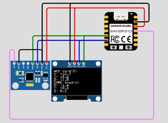
MPU6050 connected via I2C (SDA / SCL).

Program Code

// LIBRARIES
#include <Wire.h>
#include <Adafruit_GFX.h>
#include <Adafruit_SSD1306.h>
#include <Adafruit_MPU6050.h>
#include <Adafruit_Sensor.h>

// DISPLAY CONFIG
#define heigth 64 
#define width  128
#define rst   -1
Adafruit_SSD1306 oled(width,heigth,&Wire,rst);

// MPU OBJECT
Adafruit_MPU6050 mpu;

void setup() {
  
  boardBegin();

  Serial.println("Hello, XIAO ESP32-C3 BOARD!");

  oled.clearDisplay();
  oled.println("Hello, XIAO ESP32-C3 BOARD!");
  oled.display();

  delay(2000);
}

void loop() {

  sensors_event_t a, g, temp;

  // Read data from MPU6050
  mpu.getEvent(&a, &g, &temp);

  oled.clearDisplay();
  oled.setCursor(0, 0);

  // Acceleration data
  oled.println("ACC (m/s^2)");
  oled.print("X: "); oled.println(a.acceleration.x, 1);
  oled.print("Y: "); oled.println(a.acceleration.y, 1);
  oled.print("Z: "); oled.println(a.acceleration.z, 1);

  // Gyroscope data
  oled.println("GYRO (rad/s)");
  oled.print("X: "); oled.println(g.gyro.x, 1);
  oled.print("Y: "); oled.println(g.gyro.y, 1);
  oled.print("Z: "); oled.println(g.gyro.z, 1);

  oled.display();

  delay(500);
}

void boardBegin(){

  Serial.begin(115200);
  Wire.begin();

  if(!oled.begin(SSD1306_SWITCHCAPVCC, 0x3C)){
    Serial.println("Oled Display NOT Found...");
    for (;;);
  }

  oled.setTextColor(WHITE);
  oled.clearDisplay();
  oled.setTextSize(1);
  oled.setCursor(5, 5);

  // MPU initialization
  if (!mpu.begin()) {
    Serial.println("Failed to find MPU6050 chip");
    for (;;);
  }
}

Code Explanation

• Reuse of Previous Architecture: The program maintains the same structure used in previous experiments, including OLED display handling, I2C communication, and modular initialization through the boardBegin() function.
• I2C Shared Bus: Both the OLED display and the MPU6050 communicate using the I2C protocol via the Wire library. This allows multiple devices to operate on the same SDA and SCL lines.
• MPU6050 Initialization: The sensor is initialized inside boardBegin() using mpu.begin(). If the sensor is not detected, the system enters an infinite loop, which is useful for identifying hardware issues early in execution.
• Sensor Data Structure: The function mpu.getEvent() returns three structures:
  • a: acceleration (m/s²)
  • g: angular velocity (rad/s)
  • temp: internal sensor temperature
  These structures organize multi-axis data in a clean and accessible way.
• Multi-Axis Data Processing: Six variables are handled simultaneously (AX, AY, AZ, GX, GY, GZ), representing motion and rotation in 3D space. This is significantly more complex than previous single-variable sensors.
• OLED Data Visualization: The data is formatted and displayed using println(), grouping acceleration and gyroscope values separately. The use of println(value, 1) limits the output to one decimal place, improving readability on the display.
• Refresh Control: A delay of 500 ms is used to stabilize updates, preventing excessive refresh and making the data easier to read.
• ⚠️ Hardware Failure Detection: The program includes a validation step using mpu.begin(). When the sensor is not detected, the system stops execution, confirming that the issue is not related to data processing but to hardware communication.
• ⚠️ Debugging Process: Multiple tests were performed:
  • I2C scanner → no devices detected
  • Testing without OLED → no response
  • Testing on breadboard → same result
  These steps confirm that the issue is not related to wiring or PCB design.
• ⚠️ Root Cause: Since the sensor works correctly in simulation but fails in real hardware, and no I2C address is detected, the MPU6050 module is likely defective.

System in Operation

Final Reflection

This week provided a comprehensive understanding of how different types of input devices interact with a microcontroller, and how physical phenomena can be translated into digital information. Through a series of experiments, I explored both analog and digital sensors, each requiring different approaches for data acquisition and processing.

In the first experiment, using a potentiometer, I learned how analog signals are read through the ADC with 12-bit resolution, producing values between 0 and 4095. This helped me understand how continuous physical changes are converted into digital data, and how tools like the Serial Plotter can be used to visualize signal behavior in real time.

The second experiment introduced signal normalization using an analog temperature sensor. Since no absolute reference in degrees Celsius was available, I implemented a relative scale using the map() function. This allowed me to understand how calibration and scaling are essential when working with raw sensor data.

In the third experiment, using a joystick, I encountered important challenges related to interpreting input data. Initially, I incorrectly mapped the analog readings directly to position, which resulted in unstable behavior. By analyzing the problem, I understood the importance of relative control and the need for calibration and threshold filtering. This experiment highlighted how mechanical properties of input devices affect data interpretation.

The fourth experiment introduced digital sensing using the DHT22. This marked a key difference from analog sensors, as the device provides already processed data through a communication protocol. The use of external libraries simplified the implementation, but also required understanding how digital communication works. A critical hardware mistake occurred when the sensor was connected in reverse, permanently damaging it. This emphasized the importance of correct wiring and the need for protection mechanisms such as diodes in power lines.

Finally, the MPU6050 experiment introduced a more complex sensor combining multiple axes of measurement. Although the system worked correctly in simulation, the real hardware did not respond. Through systematic debugging (I2C scanning, wiring validation, and testing in different setups), I concluded that the module was defective. This reinforced the importance of validating both software and hardware independently.

Overall, this week highlighted a fundamental concept: the difference between analog and digital sensors. Analog sensors require interpretation, scaling, and noise handling, while digital sensors provide processed data but depend on communication protocols and libraries. Understanding these differences is essential for designing reliable embedded systems.

Additionally, the importance of debugging became evident throughout all experiments. Errors were not only present in code but also in hardware connections and component reliability. Learning how to systematically identify and isolate these issues is a key skill in embedded system development.

Individual Reflection – Group Assignment