Week 9: Input Devices

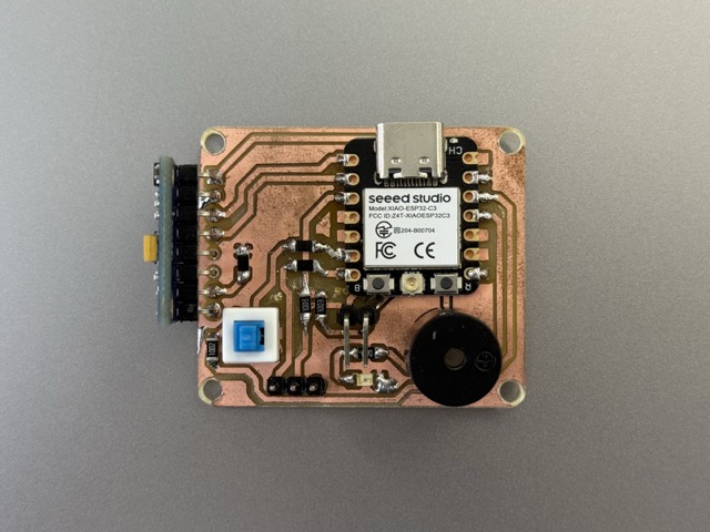
*Updated PCB with Gyroscope.

Group Assignment

Find the complete group assignment here.

Our group assignment this week was really interesting. We got to work again with measuring instruments like the oscilloscope and power supply, but the most exciting part was exploring the input devices. We spent time experimenting with a digital color-detecting sensor and an analog microphone.

The most interesting part wasn’t just using the devices, but learning how they actually work. I already understood how the color detector operated, but finding out that an analog microphone is fundamentally a capacitor was a completely new discovery for me.

Isolating the individual 1s and 0s from the color sensor on the oscilloscope was a highlight. I understood internal data flow conceptually, but seeing it graphed as distinct bit packets made it much more concrete.

Individual Assignment

Picking up from where I left last week… things seemed to be worse not very good. I quite liked my fisrt-time soldering reults, but soon after found out that some pins were placed incorrectly, to be precise SDL and SCL.

Also, on my GY-521 [gyroscope and accelerometer], I disregarded the ADO pin, which was supposed to be connected to GND for this purpose. Therefore after I had already milled the FR-1, I was advised by Onik to bridge the ADO pin with a 10kΩ resistor. Refer to more information in week 8.

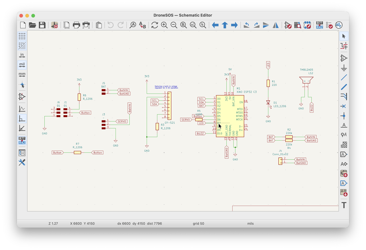
The overall schematic design look like the image below, so this week is mainly dedicated to fixing the isues from last week – designing, milling, and assembling the new PCB.

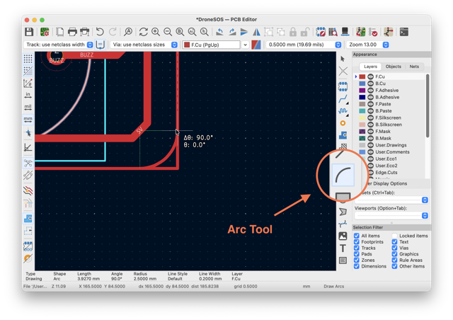
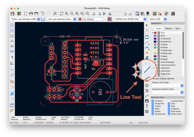
One of the key visual changes was rounding the corners. It first began with a rough draft of the layout. I outlined the box, and then put arcs [1/4th of a circle] with the Arc Tool from the right side panel [image below].

Then connected the rounded corners with Line tool.

Once the frame was achieved, I converted the shape into a common ground for the comonents [⌘ + B].

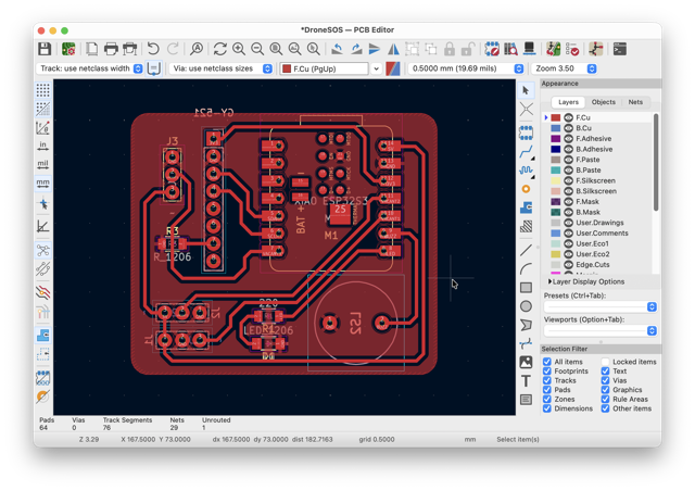
Final PCB

After some alterations, swapping places, removing extra pin headers, I was left with this final design. I added a switch button which I will program to send the device to deep sleep mode.

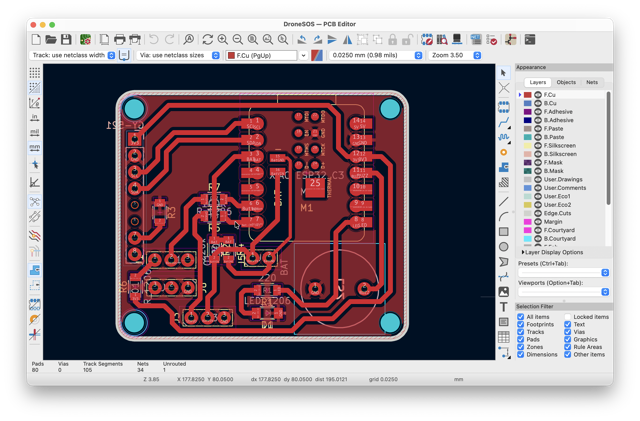
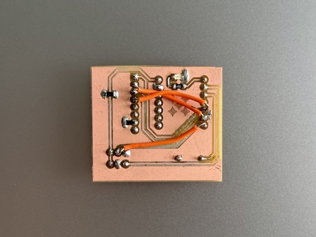
The PCB evolved from the left image into the right one.

Problem

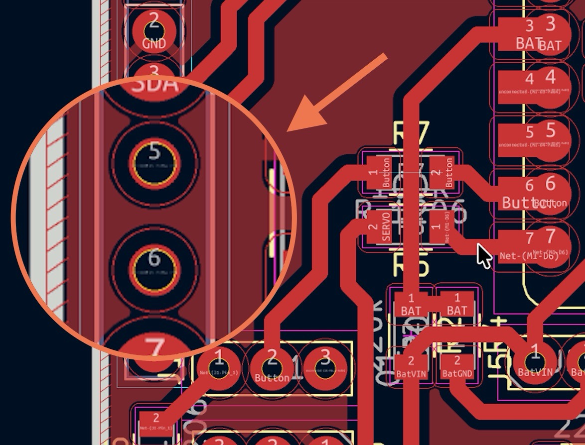
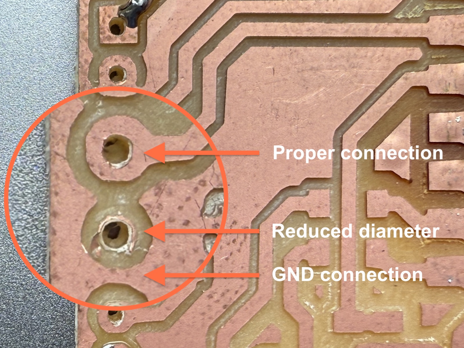
As a workaround for the isolated ground island, I narrowed the copper rings on the unused gyroscope pads. This modification created enough clearance to bridge the isolated copper and unify the ground plane. See the difference in the images below.

Intro to IMUs

An IMU, or an Inertial Measurement Unit, is a general term — not a specific product. It just means “a sensor package that measures motion and orientation using inertia,” typically by combining an accelerometer [senses linear acceleration/gravity] and a gyroscope [senses rotation rate]. Some IMUs also add a magnetometer [senses heading, like a compass] — those are sometimes called 9-axis IMUs or AHRS.

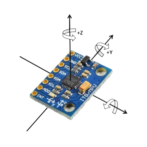So IMU is the category. Lots of different chips qualify as IMUs.

MPU6050 is one specific IMU chip, made by InvenSense. It’s a “6-axis” IMU because it packs a 3-axis accelerometer and a 3-axis gyroscope into a single chip. It talks to a microcontroller over I2C and is popular for hobby robotics, drones, and balancing projects because it’s cheap, small, and easy to wire up. Whereas the GY-521 [which I am using] is not the chip itself — it’s the name of a small breakout board that the MPU6050 chip is mounted on.

Links to purchase, and official datasheet.

How it works?

The accelerometer measures acceleration [including gravity] using tiny MEMS structures — microscopic masses that shift slightly when the chip moves or tilts. That shift is measured electrically, and since gravity always pulls down, this also tells you which way is “down.”

The gyroscope measures rotation speed on each axis [X, Y, Z], using a similar MEMS trick based on the Coriolis effect — tiny vibrating structures shift sideways when rotated, giving a rotation rate in degrees per second.

Here are two great videos which explains better, and more visually!
• Video #1
• Video #2

Gyro Implementations

I wanted something simple yet interesting – visual representation of the accelerometer’s movement on my screen. I worked with Google AI this time, and I had asked it ton write the app using Python. As I am using macOS python comes preinstalled, so all I was left to do was upload the code onto the integrated PCB, and run the code which ties the hardware with the software.

Part 1, The Firmware

The code reads raw acceleration and rotation data from an MPU6050 sensor to calculate the real-time tilt angles of an object. Because accelerometers are noisy during movement and gyroscopes drift over time, the script implements a custom 1D Kalman Filter class to mathematically fuse both streams of data. The filter continuously corrects sensor errors to output smooth, precise pitch and roll values directly to the computer via USB serial communication.

*Prompt9.1a

C++

#include <Wire.h>
#include <Adafruit_MPU6050.h>
#include <Adafruit_Sensor.h>

Adafruit_MPU6050 mpu;

#define I2C_SDA D1
#define I2C_SCL D0

// Simple 1D Kalman Filter Class
class Kalman1D {
  private:
    float Q_angle = 0.001f;   // Process noise variance for the accelerometer
    float Q_bias  = 0.003f;   // Process noise variance for the gyro bias
    float R_measure = 0.03f;  // Measurement noise variance

    float angle = 0.0f; // Reset state
    float bias  = 0.0f; // Reset bias
    float P[2][2] = {{0, 0}, {0, 0}}; // Error covariance matrix

  public:
    float update(float newAngle, float newRate, float dt) {
        // Step 1: Predict state ahead
        float rate = newRate - bias;
        angle += dt * rate;

        // Step 2: Predict error covariance ahead
        P[0][0] += dt * (dt*P[1][1] - P[0][1] - P[1][0] + Q_angle);
        P[0][1] -= dt * P[1][1];
        P[1][0] -= dt * P[1][1];
        P[1][1] += Q_bias * dt;

        // Step 3: Calculate Kalman gain
        float S = P[0][0] + R_measure;
        float K[2];
        K[0] = P[0][0] / S;
        K[1] = P[1][0] / S;

        // Step 4: Update state estimate with measurement
        float y = newAngle - angle;
        angle += K[0] * y;
        bias  += K[1] * y;

        // Step 5: Update error covariance matrix
        float P00_temp = P[0][0];
        float P01_temp = P[0][1];

        P[0][0] -= K[0] * P00_temp;
        P[0][1] -= K[0] * P01_temp;
        P[1][0] -= K[1] * P00_temp;
        P[1][1] -= K[1] * P01_temp;

        return angle;
    }
};

// Instantiate Kalman Filters
Kalman1D kalmanPitch;
Kalman1D kalmanRoll;

unsigned long lastTime = 0;

void setup() {
  Serial.begin(115200);
  Wire.begin(I2C_SDA, I2C_SCL);

  if (!mpu.begin()) {
    while (1) { delay(10); }
  }

  mpu.setAccelerometerRange(MPU6050_RANGE_4_G);
  mpu.setGyroRange(MPU6050_RANGE_250_DEG);
  mpu.setFilterBandwidth(MPU6050_BAND_21_HZ);

  lastTime = millis();
}

void loop() {
  sensors_event_t a, g, temp;
  mpu.getEvent(&a, &g, &temp);

  unsigned long currentTime = millis();
  float dt = (currentTime - lastTime) / 1000.0f;
  lastTime = currentTime;

  if (dt <= 0.0f) dt = 0.001f;

  // 1. Calculate raw angles from Accelerometer
  float rawRoll  = atan2(a.acceleration.y, a.acceleration.z) * 180.0f / PI;
  float rawPitch = atan2(-a.acceleration.x, sqrt(a.acceleration.y * a.acceleration.y + a.acceleration.z * a.acceleration.z)) * 180.0f / PI;

  // 2. Extract Gyro angular velocity rates (converted to deg/s)
  float gyroPitchRate = g.gyro.y * 180.0f / PI;
  float gyroRollRate = g.gyro.x * 180.0f / PI;

  // 3. Process measurements through the Kalman Filter
  float filteredPitch = kalmanPitch.update(rawPitch, gyroPitchRate, dt);
  float filteredRoll  = kalmanRoll.update(rawRoll, gyroRollRate, dt);

  // Stream data over USB Serial to Python
  Serial.print(filteredPitch);
  Serial.print(",");
  Serial.println(filteredRoll);

  delay(10); 
}

Part 2, The Software

The Python script creates a real-time 3D visualization window using PyGame and PyOpenGL to display the physical orientation of my PCB. It continuously listens to the specified Mac serial port to read, decode, and split the comma-separated pitch and roll data sent from the Arduino sketch [above].

In terminal I typed in the following command to install PyOpenGL:

pip3 install pyserial pygame PyOpenGL

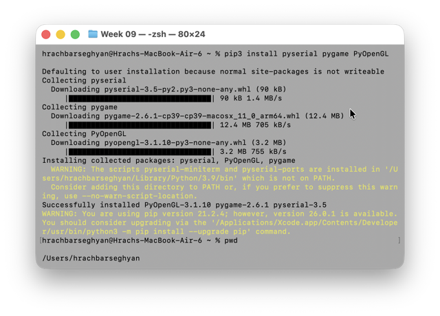
The code then applies these dynamic angle values to a colored 3D box, causing it to instantly tilt and rotate on the screen in direct synchronization with the physical accelerometer.

*Prompt9.1b

python

import sys
import serial
import pygame
from pygame.locals import *
from OpenGL.GL import *
from OpenGL.GLU import *

SERIAL_PORT = '/dev/cu.usbmodem1101' 
BAUD_RATE = 115200

# Initialize Serial Connection
try:
    ser = serial.Serial(SERIAL_PORT, BAUD_RATE, timeout=1)
except Exception as e:
    print(f"Error opening serial port: {e}")
    sys.exit()

# Define vertices and edges for a simple 3D rectangular box
vertices = (
    (1, -0.2, -1), (1, 0.2, -1), (-1, 0.2, -1), (-1, -0.2, -1),
    (1, -0.2, 1), (1, 0.2, 1), (-1, -0.2, 1), (-1, 0.2, 1)
)
edges = ((0,1), (0,3), (0,4), (2,1), (2,3), (2,7), (6,3), (6,4), (6,7), (5,1), (5,4), (5,7))
surfaces = ((0,1,2,3), (3,2,7,6), (6,7,5,4), (4,5,1,0), (1,5,7,2), (4,0,3,6))
colors = ((1,0,0), (0,1,0), (0,0,1), (1,1,0), (1,0,1), (0,1,1))

def draw_cube():
    glBegin(GL_QUADS)
    for i, surface in enumerate(surfaces):
        glColor3fv(colors[i])
        for vertex in surface:
            glVertex3fv(vertices[vertex])
    glEnd()

    glColor3fv((0,0,0)) # Black outlines
    glBegin(GL_LINES)
    for edge in edges:
        for vertex in edge:
            glVertex3fv(vertices[vertex])
    glEnd()

def main():
    pygame.init()
    display = (800, 600)
    pygame.display.set_mode(display, DOUBLEBUF | OPENGL)
    pygame.display.set_caption("XIAO ESP32-C3 3D IMU Visualizer")

    gluPerspective(45, (display[0]/display[1]), 0.1, 50.0)
    glTranslatef(0.0, 0.0, -5.0)

    pitch, roll = 0.0, 0.0

    while True:
        for event in pygame.event.get():
            if event.type == pygame.QUIT:
                ser.close()
                pygame.quit()
                sys.exit()

        # Read serial data from ESP32
        if ser.in_waiting > 0:
            try:
                line = ser.readline().decode('utf-8').strip()
                data = line.split(',')
                if len(data) == 2:
                    pitch = float(data[0])
                    roll = float(data[1])
            except:
                pass # Ignore corrupt/incomplete serial packets

        # Rendering
        glClear(GL_COLOR_BUFFER_BIT | GL_DEPTH_BUFFER_BIT)
        glEnable(GL_DEPTH_TEST)

        glPushMatrix()
        # Apply rotations matching the IMU physics
        glRotatef(pitch, 1, 0, 0)
        glRotatef(roll, 0, 0, 1)

        draw_cube()
        glPopMatrix()

        pygame.display.flip()
        pygame.time.wait(10)

if __name__ == '__main__':
    main()

Conclusion

I was not very please with the results. While I was excited for the simple graphics, the system captured too much noise. However, the visualization gave birth to ideas for other applications, particularly how this technology could enhance gyroscope-based perception.

References

• PCB ZIP

• Part 1, C++
• Part 2, Python

Prompts

Prompt9.1 Create a Python application on macOS that visualizes 3D movement using data from an MPU6050 [GY-521] IMU. The hardware configuration connects SDA to D1, SCL to D0, VCC to 3.3V, and GND to GND. The software should render a simple 3D geometric shape on-screen that accurately mirrors the real-time physical movement and rotation of the gyroscope.