15. Wildcard Week

What did I do this week?

Artificial intelligence (AI) is a field of computer science that seeks to create systems capable of performing tasks that, until recently, required human intelligence. These tasks include pattern recognition, learning, planning, and natural language understanding, among others. One of the most promising and effective approaches within AI is the use of artificial neural networks.

Artificial Neural Networks

Artificial neural networks are computational models inspired by the functioning of the human brain. These models are designed to simulate the way the brain processes information. They consist of a set of nodes, known as “neurons”, organized in layers, which are interconnected by “synapses”. Each connection has a weight that is adjusted during model training.

Key Components of Neural Networks

1. Neurons: These are the basic processing units of a neural network. Each neuron receives various inputs, adds them in a weighted manner based on their weights, and then applies an activation function to generate its output.
2. Weights and Biases: These are parameters of the neural network. The weights control the importance of the inputs to each neuron, while the biases allow the output to be adjusted along with the activation function without relying exclusively on the inputs.
3. Activation Function: This is a mathematical function applied to the output of each neuron. It defines the threshold at which that neuron will be activated. The most common activation functions include ReLU, sigmoid and tanh.
4. Layers of a Neural Network:
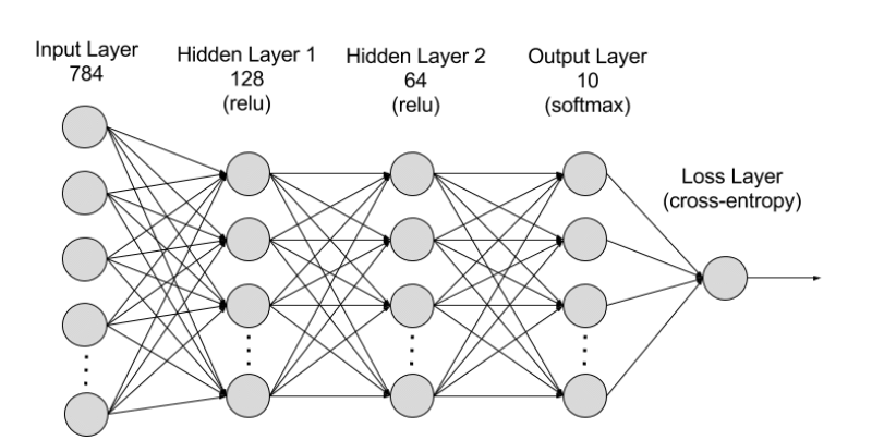
   1. Input Layer: Receives input data from the model.
   2. Hidden Layers: These are layers that lie between the input and output. They allow the network to learn more complex characteristics.
   3. Output Layer: Produces the final result of the model. The activation function in this layer depends on the type of problem (e.g., softmax for classification).
5. Hidden Layers: These are layers that are neither input nor output. Each neuron in a hidden layer performs a weighted sum of all inputs, applies an activation function and passes the result to the next layer. Hidden layers are essential for the network to learn complex representations of the data.

Neural Network Training

Training a neural network is a crucial process to adjust the parameters (weights and biases) of the model to minimize the prediction error. This process is performed through several iterative and systematic steps to gradually improve the accuracy of the model.

Phases of the Training Process

Initialization of Weights and Biases:
• Before training begins, we initialize the weights and biases of the network. These can be initialized randomly or by some more sophisticated method to help the convergence of the model.


Forward Propagation:
• Each input of the training set is passed through the network, layer by layer, from the input layer to the output layer.
• At each neuron, a weighted sum of the inputs is performed using the weights and biases, and the result is passed through an activation function to obtain the output of the neuron.


Error Calculation (Loss Function):
• Once the network predictions are obtained, the error is calculated by comparing the network output with the expected output (true label). This error is measured using a loss function (such as mean square error for regression or cross-entropy for classification).


Backpropagation:
• In this step, the gradient of the loss function with respect to each weight and bias in the network is calculated by calculating partial derivatives.
• This gradient indicates how each weight and bias should be adjusted to minimize the error.
• Chain rules are used to propagate these gradients back through the network from output to input.


Updating Weights and Biases (Gradient Descent):
• Using the gradient computed in the backpropagation step, the weights and biases are adjusted, generally in the direction that minimizes error.
• The rate at which these adjustments are made is controlled by a parameter called “learning rate”.


Iteration through Epochs and Batches:
• Epoch: A complete cycle over the entire training data set.
• Batch Size: Number of training samples seen before making an update to the weights. This defines how large a step is taken in the gradient descent.
• At each epoch, the training data is usually divided into multiple “batches” or batches.
• The steps of forward propagation, error calculation, backpropagation and weight update are repeated for each batch.


Evaluation and Tuning:
• After each epoch, it is common to evaluate the model on a validation data set to see how it is generalizing to new data.
• This process helps to detect if the model is overfitting or underfitting and allows for adjustments such as modifying the learning rate or changing the model architecture.

Important Terms in Neural Networks

• Normalization: Adjustment of the input values to a common scale to make training more efficient.
• Loss Function: A measure of how different the model predictions are from the actual labels.
• Optimizer: Method for changing neural network attributes such as weights and learning rate to reduce losses.
• Epochs: Complete cycle over the training data set.
• Batch Size: Number of data samples seen by the model in an iteration within an epoch before updating the weights.
• Overfitting and Underfitting: Overfitting occurs when a model learns too much about the training data and does not generalize well. Underfitting occurs when a model does not learn enough from the training data.

Let's get to practice!

For this assignment I implemented the use of neural networks using python. One of the most powerful frameworks for working with neural networks in Python is TensorFlow. Developed by Google, TensorFlow allows the creation, training and evaluation of a wide variety of machine learning models with remarkable efficiency and scalability. TensorFlow's integration with Keras, a high-level API, facilitates the construction of neural networks by abstracting away the more complex operations, allowing users to focus on model design rather than low-level implementation details.

To show how these tools can be applied to practical machine learning problems, I used the Fashion MNIST dataset, a popular resource for getting started in computer vision. This dataset contains 70,000 grayscale images of 10 clothing categories, divided into 60,000 images for training and 10,000 for testing. Each image has a resolution of 28x28 pixels, making them manageable for model training without compromising the complexity of the classification problem. Using this set, I built a neural network model to identify and classify different categories of clothing, a process that includes image normalization, model architecture definition, training and final evaluation.

1. Import of libraries

    import tensorflow as tf  
    import pandas as pd  
    import matplotlib.pyplot as plt  
    import numpy as np  
    import random  

First, we import the necessary libraries.

• TensorFlow (tf): An open source machine learning library developed by Google for building and training neural networks. It allows the creation of deep learning models and other ML algorithms in an efficient and scalable way.
• Pandas (pd): Used for data manipulation and analysis. Provides data structures and operations for manipulating numerical tables and time series.
• Matplotlib (plt): A Python data visualization library, which provides a MATLAB-like way of graphing. It allows you to create high-quality graphs and data visualizations.
• NumPy (np): Essential for numerical computation in Python. Provides vector and matrix data structures, along with a large collection of mathematical functions to operate on these objects.
• Random: Used to generate random numbers. Can be useful for randomly selecting data, for shuffling or random initialization of weights in neural network models.

2. Data Loading

    mnist = tf.keras.datasets.fashion_mnist
    (x_train, y_train), (x_test, y_test) = mnist.load_data()  # x -> imágenes, y -> etiquetas

• tf.keras.datasets.fashion_mnist: Loads the Fashion MNIST dataset directly from TensorFlow Keras. This dataset contains clothing images classified into 10 categories.
• (x_train, y_train), (x_test, y_test): Splits the dataset into images and labels for training and testing. x_train and x_test contain the clothing images, while y_train and y_test contain the labels corresponding to these images.

3. Display of a Random Image

    class_names = ["T-shirt/top", "Trouser", "Pullover", "Dress", "Coat", "Sandal", "Shirt", "Sneaker", "Bag", "Ankle boot"]
    n = random.randint(0, len(x_train))
    plt.imshow(x_train[n], cmap="gray")
    plt.title(f'n = {n}')
    plt.xlabel(f'Class: {class_names[y_train[n]]}')
    plt.show()

• class_names: List of class labels for Fashion MNIST, used to map numeric labels to clothing names.
• random.randint(0, len(x_train)): Selects a random index to display an image.
• plt.imshow(): Displays an image. cmap="gray" indicates that the image is in grayscale.
• plt.title() and plt.xlabel(): Set the title and x-axis label of the graphic to display relevant image information.

4. Data normalization

    x_train, x_test = x_train / 255.0, x_test / 255.0

5. Model Architecture Definition

    model = tf.keras.models.Sequential([
        tf.keras.layers.Flatten(input_shape=(28, 28)),
        tf.keras.layers.Dense(128, activation='relu'),
        tf.keras.layers.Dense(64, activation='relu'),
        tf.keras.layers.Dense(32, activation='relu'),
        tf.keras.layers.Dense(16, activation='relu'),
        tf.keras.layers.Dense(10, activation='softmax')
    ])

• model = tf.keras.models.Sequential([...]): Defines a sequential model in TensorFlow Keras. This type of model is a linear stack of layers, which means that each layer has exactly one input tensor and one output tensor.
• tf.keras.layers.Flatten(input_shape=(28, 28)): The first layer of the model is a Flatten layer that converts each 28x28 pixel input image into a 784 pixel flat array (28*28). This transforms the image structure so that it can be processed by the subsequent dense layers.
• tf.keras.layers.Dense(128, activation='relu'): This is a dense layer with 128 neurons. The activation function ReLU (Rectified Linear Unit) is used here to introduce nonlinearity into the model, allowing the network to learn more complex patterns.
• tf.keras.layers.Dense(64, activation='relu'): Another dense layer, this time with 64 neurons, also using ReLU as activation function.
• tf.keras.layers.Dense(32, activation='relu'): Continues with a dense layer of 32 neurons, keeping the ReLU activation function.
• tf.keras.layers.Dense(16, activation='relu'): A dense layer with 16 neurons. Like the previous ones, it uses ReLU for activation.
• tf.keras.layers.Dense(10, activation='softmax'): The last layer is a dense layer with 10 neurons, one for each clothing class in the Fashion MNIST dataset. The activation function softmax is used here to obtain a probability distribution over the 10 classes, facilitating classification.

6. Model Compilation

    model.compile(
        optimizer='adam',
        loss='sparse_categorical_crossentropy',
        metrics=['accuracy']
    )

• model.compile(): Configures the model for training.
• optimizer='adam': The Adam optimizer is used to update the weights of the network based on the gradient of the loss function.
• loss='sparse_categorical_crossentropy': This is the loss function used for multiclass classification problems. It measures how different the distributions of the true labels and the model predictions are.
• metrics=['accuracy']: List of metrics to be evaluated by the model during training and testing. Here, we use accuracy, the fraction of correctly classified images.

7. Model Training

    model_history = model.fit(
        x_train, 
        y_train, 
        epochs=25, 
        validation_data=(
            x_test, 
            y_test
        )
    )

• model.fit(): Trains the model with the input data.
• x_train and y_train: are the training data (images and labels, respectively).
• epochs=25: indicates that the model must pass through the entire training dataset 25 times.
• validation_data=(x_test, y_test): allows the model to evaluate the loss and metrics in the validation data (in this case, the test set) at the end of each epoch.

8. Evaluation of the Model

    test_loss, test_acc = model.evaluate(x_test, y_test)
    print(f"Loss = {test_loss}, Accuracy = {test_acc}")

• model.evaluate(): Evaluates the performance of the model with the test data after training. Returns the loss and accuracy or any other metric specified in model.compile().
• print(): Displays the loss (test_loss) and accuracy (test_acc) of the model on the test set.

9. Loss Visualization During Training and Validation

    plt.plot(
        model_history.history['loss'], 
        label='Training Loss'
    )
    plt.plot(
        model_history.history['val_loss'], 
        label='Validation Loss'
    )
    plt.title("Model Loss Over Epochs")
    plt.xlabel("Epoch")
    plt.ylabel("Loss")
    plt.legend()
    plt.show()

• plt.plot(model_history.history.history['loss'], label='Training Loss'): This line plots the training loss stored in model_history.history['loss'] over the epochs. Use the label 'Training Loss' for this data series in the plot.
• plt.plot(model_history.history['val_loss'], label='Validation Loss'): Similar to the previous line, but for the validation loss model_history.history['val_loss']. This data series is labeled as “Validation Loss”.
• plt.title("Model Loss Over Epochs"): Sets the title of the graph, which in this case is “Model Loss Over Epochs”, to indicate that it is showing how the model loss changes with each epoch.
• plt.xlabel("Epoch") and plt.ylabel("Loss"): These lines set the labels for the X and Y axes of the graph. “Epoch” is the label for the X-axis and “Loss” is the label for the Y-axis.
• plt.legend(): Adds a legend to the chart. Because the data series have labels (“Training Loss” and “Validation Loss”), this legend provides useful context to identify each line in the chart.
• plt.show(): Displays the graph with all presets applied. This is the command that creates the visualization based on the data and settings provided.

10. Model Saving

    model.save("fashion_mnist.h5")

• model.save(): Saves the trained model in the file “fashion_mnist.h5”. This file contains the model architecture, weights and training settings. This allows to load the model later to make predictions without retraining.

Testing the model with dataset data

    import tensorflow as tf
    import numpy as np
    import matplotlib.pyplot as plt
    import random
    import seaborn as sns

    # Load pre-trained model from 'fashion_mnist.h5'
    model = tf.keras.models.load_model('fashion_mnist.h5')

    # Load Fashion MNIST dataset
    fashion_mnist = tf.keras.datasets.fashion_mnist
    (x_train, y_train), (x_test, y_test) = fashion_mnist.load_data()

    # Define class names for Fashion MNIST
    class_names = ["T-shirt/top", "Trouser", "Pullover", "Dress", "Coat", "Sandal", "Shirt", "Sneaker", "Bag", "Ankle boot"]

    # Select a random image index from the test set
    n = random.randint(0, len(x_test))

    # Normalize test images
    x_test = x_test / 255.0

    # Make predictions on test images
    predictions = model.predict(x_test)

    # Calculate the confusion matrix
    conf_matrix = tf.math.confusion_matrix(y_test, np.argmax(predictions, axis=1))
    print(conf_matrix)

    # Plot the confusion matrix as a heatmap
    sns.heatmap(conf_matrix, annot=True, fmt='d', cmap='coolwarm')
    plt.xlabel('Predicted')
    plt.ylabel('Real')
    plt.show()

    # Display the randomly selected test image
    plt.imshow(x_test[n], cmap='binary_r')
    plt.xlabel(f'Real: {class_names[y_test[n]]}, Pred: {class_names[np.argmax(predictions[n])]}')
    plt.show()

1. Load Libraries and Model:
   We import necessary libraries like TensorFlow, NumPy, Matplotlib, and Seaborn. Then we load a pre-trained neural network model named fashion_mnist.h5 using TensorFlow's Keras API.
2. Load Dataset:
   The Fashion MNIST dataset is loaded using TensorFlow's built-in dataset functionality. It's divided into training and testing sets, each containing images and their corresponding labels.
3. Define Class Names:
   We define a list called class_names containing the names of different clothing items. These will be used later for interpretation and visualization of the predictions.
4. Select Random Image:
   We randomly select an index (n) from the test set. This index will be used to display a random test image later.
5. Normalize Test Images:
   Pixel values of the test images are normalized to be between 0 and 1. This is a standard preprocessing step for neural network models.
6. Make Predictions:
   The pre-trained model is used to make predictions on the normalized test images. These predictions are stored in the predictions variable.
7. Calculate Confusion Matrix:
   We calculate the confusion matrix to evaluate the performance of the model. The confusion matrix compares the true labels (y_test) with the predicted labels (np.argmax(predictions, axis=1)).
8. Plot Confusion Matrix:
   The confusion matrix is visualized as a heatmap using Seaborn's heatmap function. This provides a clear representation of how well the model is performing across different classes.
9. Display Random Test Image:
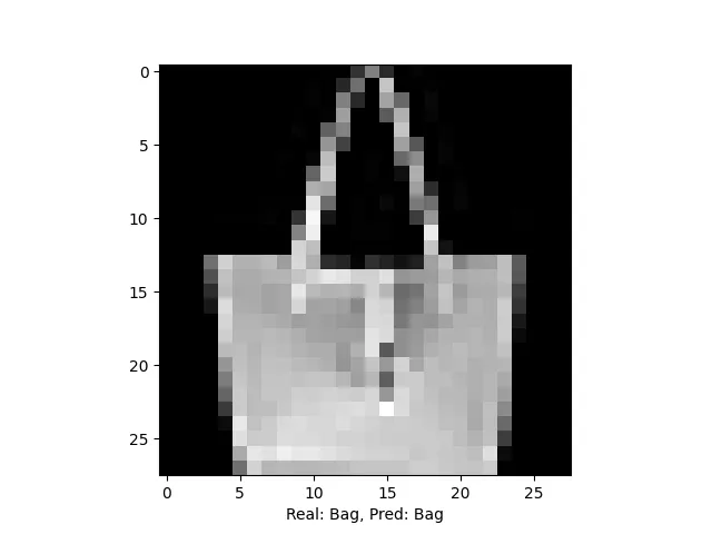
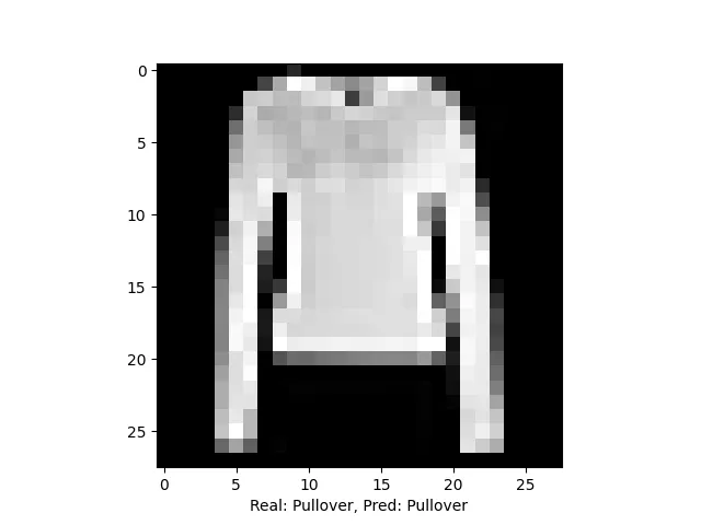
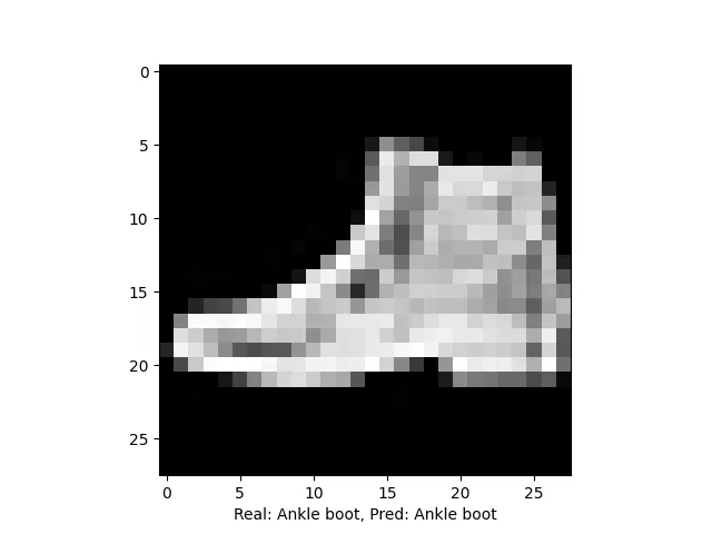
   We display a randomly selected test image along with its true label and the label predicted by the model. This helps us understand how well the model is generalizing to unseen data.

Some examples

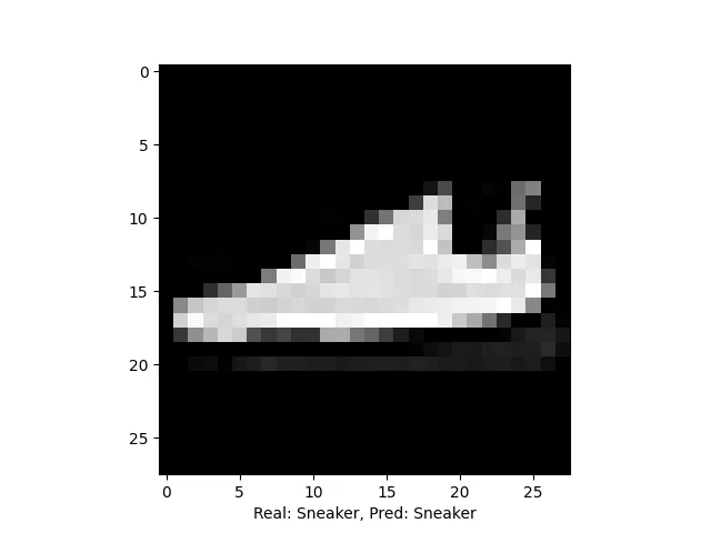
Testing the model with real images

    import tensorflow as tf
    import numpy as np
    import matplotlib.pyplot as plt
    from PIL import Image  # Python Imaging Library for image manipulation

    # Load the pre-trained model from 'fashion_mnist.h5'
    model = tf.keras.models.load_model('fashion_mnist.h5')

    # Class names for the Fashion MNIST dataset
    class_names = ["T-shirt/top", "Trouser", "Pullover", "Dress", "Coat", "Sandal", "Shirt", "Sneaker", "Bag", "Ankle boot"]

    # Load and process the image for prediction
    img = Image.open('imagenes/ankle_boat2.jpg')  # Open the image
    img = img.convert('L')  # Convert to grayscale
    img = img.resize((28, 28))  # Resize to 28x28 pixels
    img = Image.fromarray(255 - np.array(img))  # Invert colors
    img = np.array(img)  # Convert to NumPy array
    img = img / 255.0  # Normalize pixel values
    img = img.reshape(1, 28, 28)  # Reshape for model input

    # Make a prediction
    prediction = model.predict(img)
    label_pred = class_names[np.argmax(prediction)]  # Get class with highest probability

    # Display the image and predicted label
    plt.imshow(img[0], cmap='binary_r')  # Show image in grayscale
    plt.title(f"Predicted: {label_pred}")  # Show predicted label
    plt.show()  # Display the figure

1. Load Libraries and Model:
   • TensorFlow, NumPy, Matplotlib, and PIL (Python Imaging Library) are imported.
   • The pre-trained model named fashion_mnist.h5 is loaded using TensorFlow's Keras API.
2. Define Class Names:
   • A list called class_names is defined, containing the names of different clothing items in the Fashion MNIST dataset.
3. Load and Process Image:
   • An image named 'imagenes/ankle_boat2.jpg' is loaded using PIL's Image.open() function.
   • The image is converted to grayscale using the convert('L') method.
   • It's resized to 28x28 pixels, which is the input size expected by the model.
   • Colors are inverted by subtracting the pixel values from 255.
   • The image is converted to a NumPy array and pixel values are normalized to be between 0 and 1.
   • The image is reshaped to have a single channel (necessary for model input) using reshape().
4. Make Prediction:
   • The pre-trained model predicts the class probabilities for the input image using model.predict(img).
5. Get Predicted Label:
   • The index of the class with the highest probability is extracted using np.argmax(prediction).
   • The corresponding class name from class_names is retrieved using this index.
6. Display Image and Prediction:
   • The grayscale image is displayed using Matplotlib's imshow() function.
   • The predicted label is displayed as the title of the figure.

Some examples

The following images are the actual images I used.

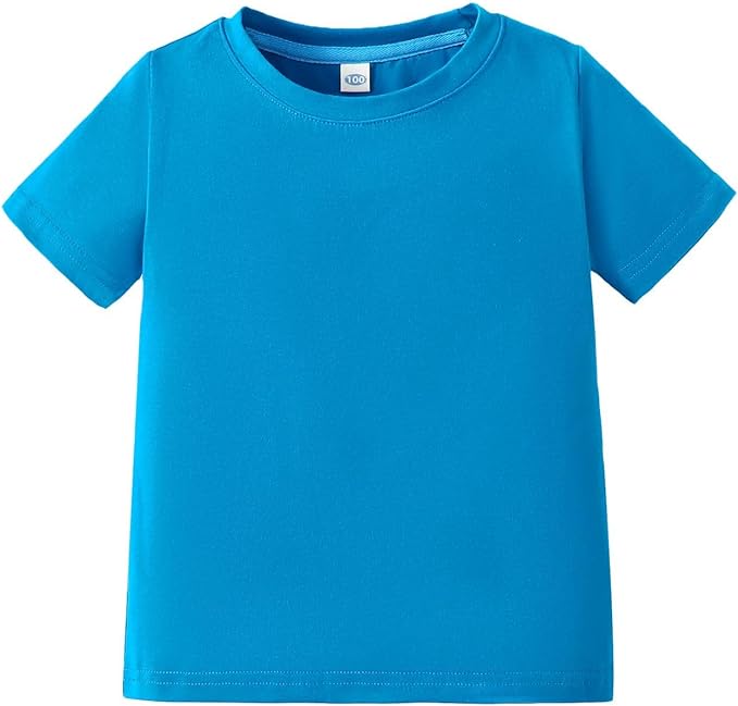
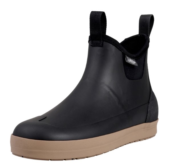
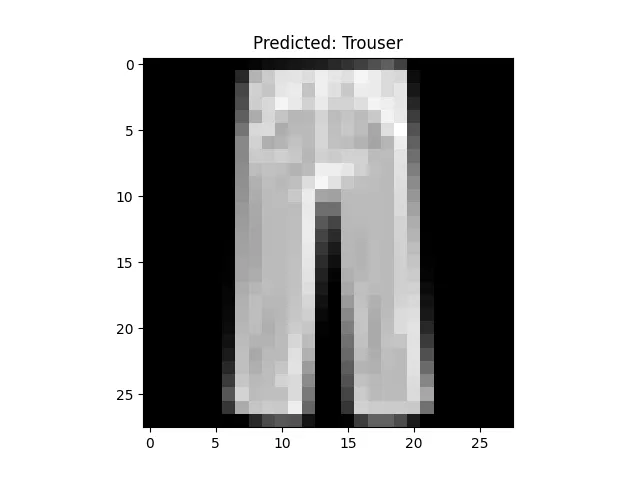
The others below are the predictions made by my model.

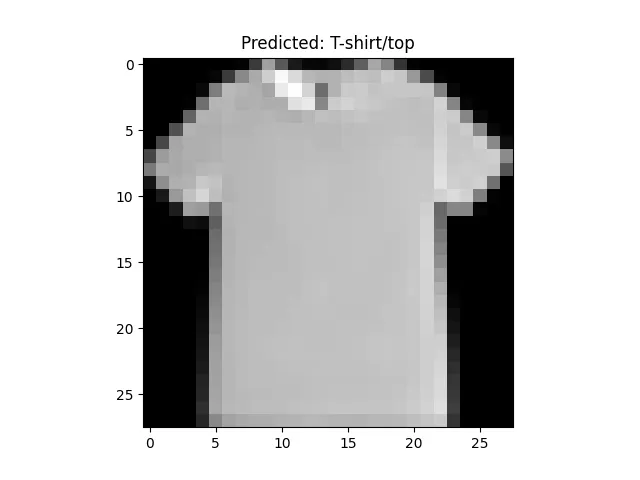
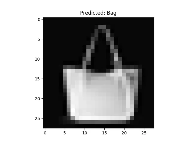
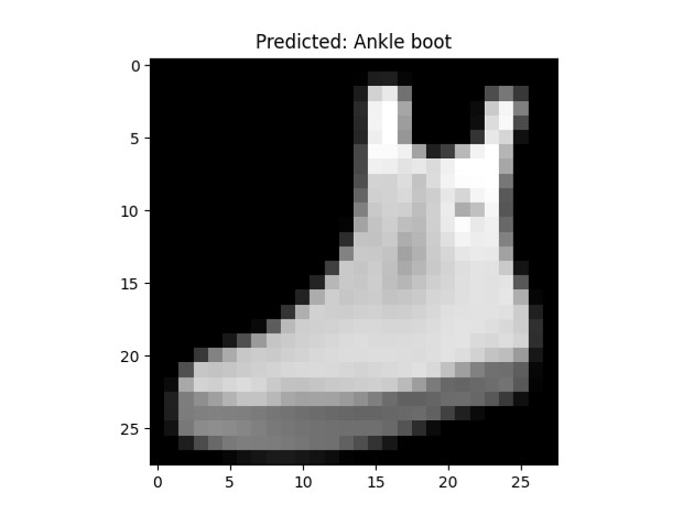
Real-time model testing

Finally, another way to test the model is in real time. Fortunately Python includes several tools to facilitate this process, below is the code and an explanation of it.

    import cv2
    import numpy as np
    import tensorflow as tf

    # Load pre-trained model
    model = tf.keras.models.load_model('fashion_mnist.h5')

    # Classes of objects that the model can detect
    class_names = ["T-shirt/top", "Trouser", "Pullover", "Dress", "Coat", "Sandal", "Shirt", "Sneaker", "Bag", "Ankle boot"]

    # Initialize video capture from the first available camera
    cap = cv2.VideoCapture(0)

    while True:
        # Capture frame by frame
        ret, frame = cap.read()

        if not ret:
            print("Failed to grab frame")
            break

        # Preprocess the frame for the model (this process may vary based on your model)
        img = cv2.cvtColor(frame, cv2.COLOR_BGR2GRAY)  # Convert to grayscale
        img = cv2.resize(img, (28, 28))  # Resize to 28x28 like Fashion MNIST model
        img = img / 255.0  # Normalize
        img = img.reshape(1, 28, 28)  # Reshape for the model

        # Make prediction using the model
        predictions = model.predict(img)
        predicted_class = class_names[np.argmax(predictions)]  # Get class with highest probability

        # Display text on the frame
        cv2.putText(frame, 
                    f"Predicted: {predicted_class}", 
                    (50, 50), 
                    cv2.FONT_HERSHEY_SIMPLEX, 
                    1, 
                    (255, 255, 255), 
                    2, 
                    cv2.LINE_AA)

        # Show the resulting frame
        cv2.imshow('Video', frame)

        # Break if 'q' is pressed
        if cv2.waitKey(1) & 0xFF == ord('q'):
            break

    # When everything is done, release the capture
    cap.release()
    cv2.destroyAllWindows()

1. Import Libraries:
   • cv2, numpy, and tensorflow libraries are imported. These are used for working with images, arrays, and machine learning tasks respectively.
2. Load Pre-trained Model:
   • The pre-trained neural network model named fashion_mnist.h5 is loaded using TensorFlow's Keras API.
3. Define Class Names:
   • A list called class_names is defined, containing the names of different clothing items that the model can predict.
4. Initialize Video Capture:
   • Video capture is initialized from the first available camera. The 0 in cv2.VideoCapture(0) indicates the default camera.
5. Video Capture Loop:
   • A while loop is started to continuously capture frames from the video feed.
6. Capture Frame:
   • Each iteration of the loop captures a frame (frame) from the video feed.
7. Preprocess Frame for Model:
   • The captured frame is preprocessed to prepare it for input to the model.
   • The frame is converted to grayscale, resized to 28x28 pixels (matching the Fashion MNIST model input size), and normalized to have pixel values between 0 and 1.
   • The shape of the frame is changed to (1, 28, 28) to match the input shape expected by the model.
8. Make Prediction:
   • The preprocessed frame is fed into the model to make predictions.
   • The model predicts class probabilities for the input frame, and the class with the highest probability is selected as the predicted class.
9. Display Prediction on Frame:
   • The predicted class is displayed as text on the frame using cv2.putText() function.
   • The text is positioned at coordinates (50, 50) with a white color and font size 1.
10. Show Frame:
    • The resulting frame with the predicted class text is displayed in a window titled 'Video' using cv2.imshow() function.
11. Quit the Loop:
    • The loop continues until the user presses the 'q' key.
    • If the 'q' key is pressed, the loop breaks, and the video capture is released.
12. Release Resources:
    • After the loop exits, the video capture is released using cap.release() to free up the camera resources.
    • All OpenCV windows are closed using cv2.destroyAllWindows().

The following image is a test of how the model works in real time.

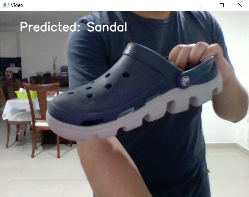
Something easier to do?

Google's Teachable Machine is a web tool developed to democratize learning artificial intelligence technologies, making it easy to create custom machine learning models without writing code. Specially designed for beginners in the field of AI, it allows users to train image, sound or pose classification models by simply using a graphical user interface.

Teachable Machine Main Features

How to use this tool?

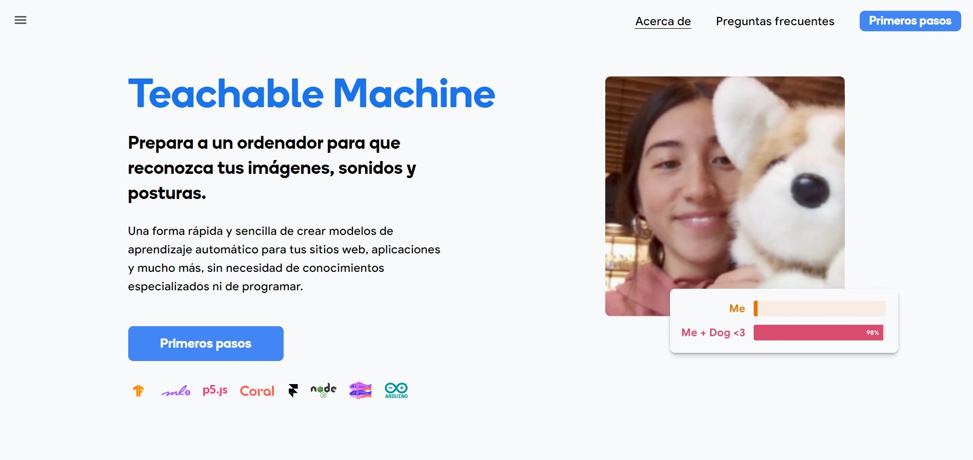
1. The first step is to open Teachable Machine in our browser. You can open it in the following link. Then click on the First steps option to get started.

2. This tool offers us to make three different projects, the first one is an image sorter, the second one is based on audio and the last one is based on postures. The one I used for this practice was the image project.

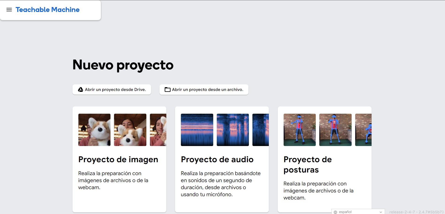
3. After selecting image project, select the standard image template option, the other inserted image template option works for microcontrollers.

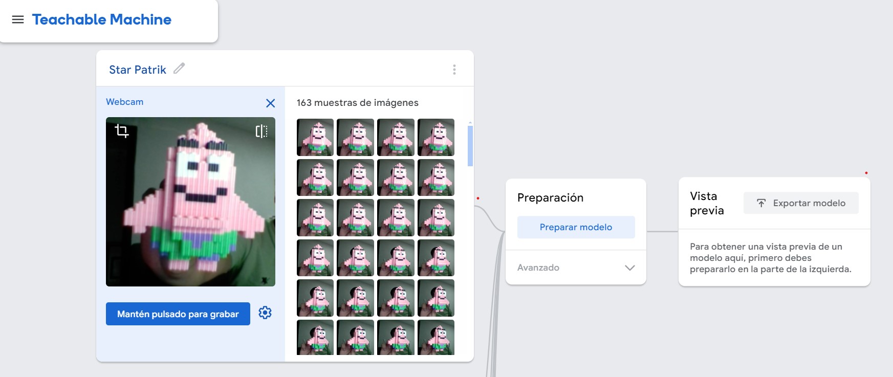
4. To start generating the model we have to prepare our data set. Since I have several figures I decided to make a classifier of different figures. The image below shows several options, we will start with the option to add a class. Each image will have a different class. Adding a class will activate our computer camera and we will be able to take a video of each figure. This tool will convert the video to images and will indicate how many images we have of each shape. The more images and in different positions the better for the model. We can also change the name of each class.

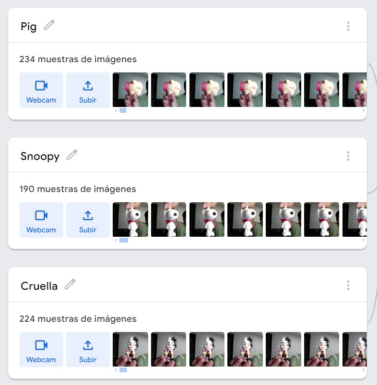
5. In total I made 7 classes, that is, I used 7 figures for my classifier. These are the figures I used:
- Patrick Star
- Goku
- Deku
- A pig
- Snoopy
- Cruella
- Venom

6. The next step is to prepare the model. We can leave the settings that the tool comes with by default or change them in the Advanced part. Here we can change the epochs, the batch size and the learning rate.

7. After waiting for the model to be ready we will have the following preview to test the model.

8. Finally, we can export the model for use elsewhere. I exported it in .js to put it on my site.

Result

Press the button to start

The following video is a sample of how the model works.

Files