9. Input Devices

This week we had to:

• Probe an input device’s analog levels and digital signals

Gyumri lab

This week, under the guidance of Onik Babajanyan, we used an oscilloscope to measure analog and digital signals from input devices connected to our PCB.

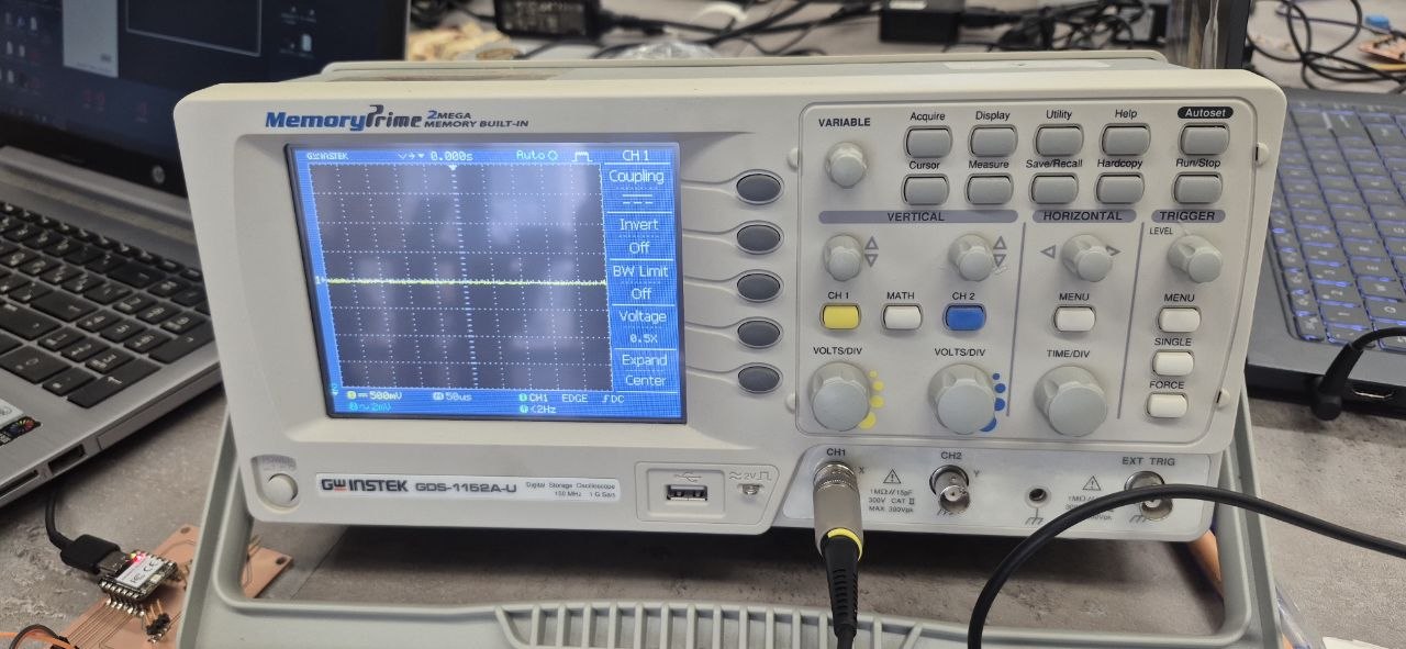
Experiment 1: Potentiometer (Analog Pin)

We applied voltage to the analog pin of a potentiometer. As we rotated it, the waveform on the screen rose and fell smoothly in proportion to the movement — a continuous, gradual change.

Experiment 2: Photoresistor (Digital Pin)

We connected the oscilloscope to the digital pin of a photoresistor. Switching the light on and off produced sharp, immediate transitions on the screen — the signal jumping between high and low with no in-between.

Experiment 3: Photoresistor (Analog Pin)

We repeated the light test using the analog pin instead. This time the transitions were smooth, similar to what we observed with the potentiometer.

Conclusion

Analog signals change continuously, reflecting gradual shifts in input. Digital signals switch abruptly between two discrete states. Seeing both behaviors on the oscilloscope made the difference between them concrete rather than just theoretical.

🔬 Dilijan Lab — Mariam & Hrach

---

Experiment 1 — Microphone on Breadboard

Before we started, our instructor Onik asked us: “What components do you need to connect a microphone to an oscilloscope on a breadboard, and why?”

This pushed us to think about the circuit before building it, not just wire things up blindly.

What We Needed to Understand First

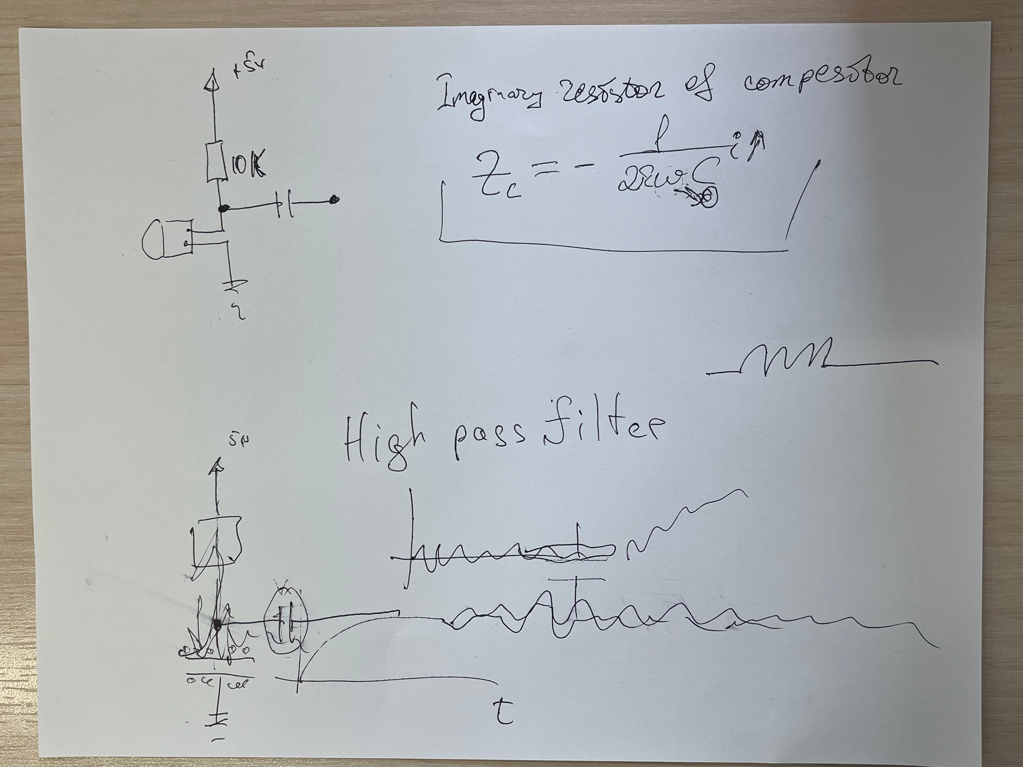
Imaginary Resistor of a Capacitor (Capacitive Reactance)

Onik explained that a capacitor does not behave like a simple resistor — it has an imaginary resistance that depends on frequency. This is called capacitive reactance, written as:

Zc = -1 / (2π · f · C)

This means: - At high frequencies (like voice or sound), the capacitor has low resistance — it passes the signal through easily. - At low frequencies or DC, it has high resistance — it blocks the signal.

This is exactly why we use a capacitor in our microphone circuit: to block the DC bias voltage while letting the AC audio signal pass through to the oscilloscope.

High Pass Filter

The capacitor also acts as a high pass filter — it lets high-frequency signals (sound waves) through while blocking the DC offset. Without it, the oscilloscope would see a flat DC line with a tiny signal on top. With it, you see only the clean AC audio waveform.

Circuit We Built

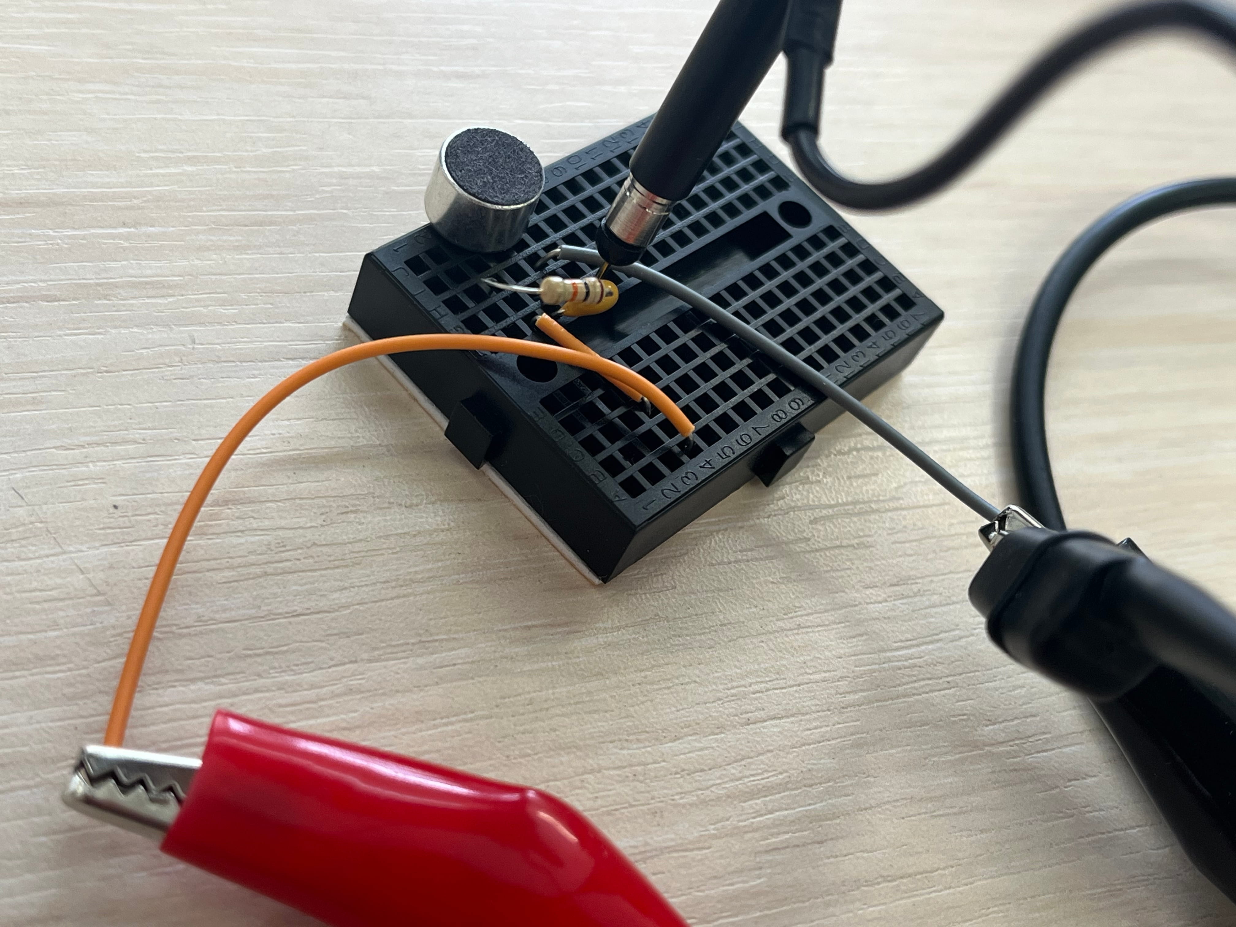
We connected the microphone (HMO1003A-65 electret capsule) on a mini breadboard with two components:

• 10 kΩ resistor — bias resistor connecting the mic output pin to 5V, providing the DC current the mic’s internal FET needs to operate
• Coupling capacitor — blocks the DC voltage so only the audio AC signal reaches the oscilloscope probe

Result

When we spoke or made noise near the microphone, the oscilloscope showed audio pulses — irregular waveforms that responded directly to the sound. In silence, the trace returned to a flat line. This confirmed that the coupling capacitor was correctly removing the DC bias and passing only the AC audio signal through.

What We Learned

The microphone circuit taught us two things at once: that electret mics need a DC bias to work, and that a capacitor’s frequency-dependent imaginary resistance (Zc) makes it the right tool to separate that DC bias from the AC audio signal we actually want to measure.

---

Experiment 2 — TCS34725 Colour Sensor + I2C on Oscilloscope

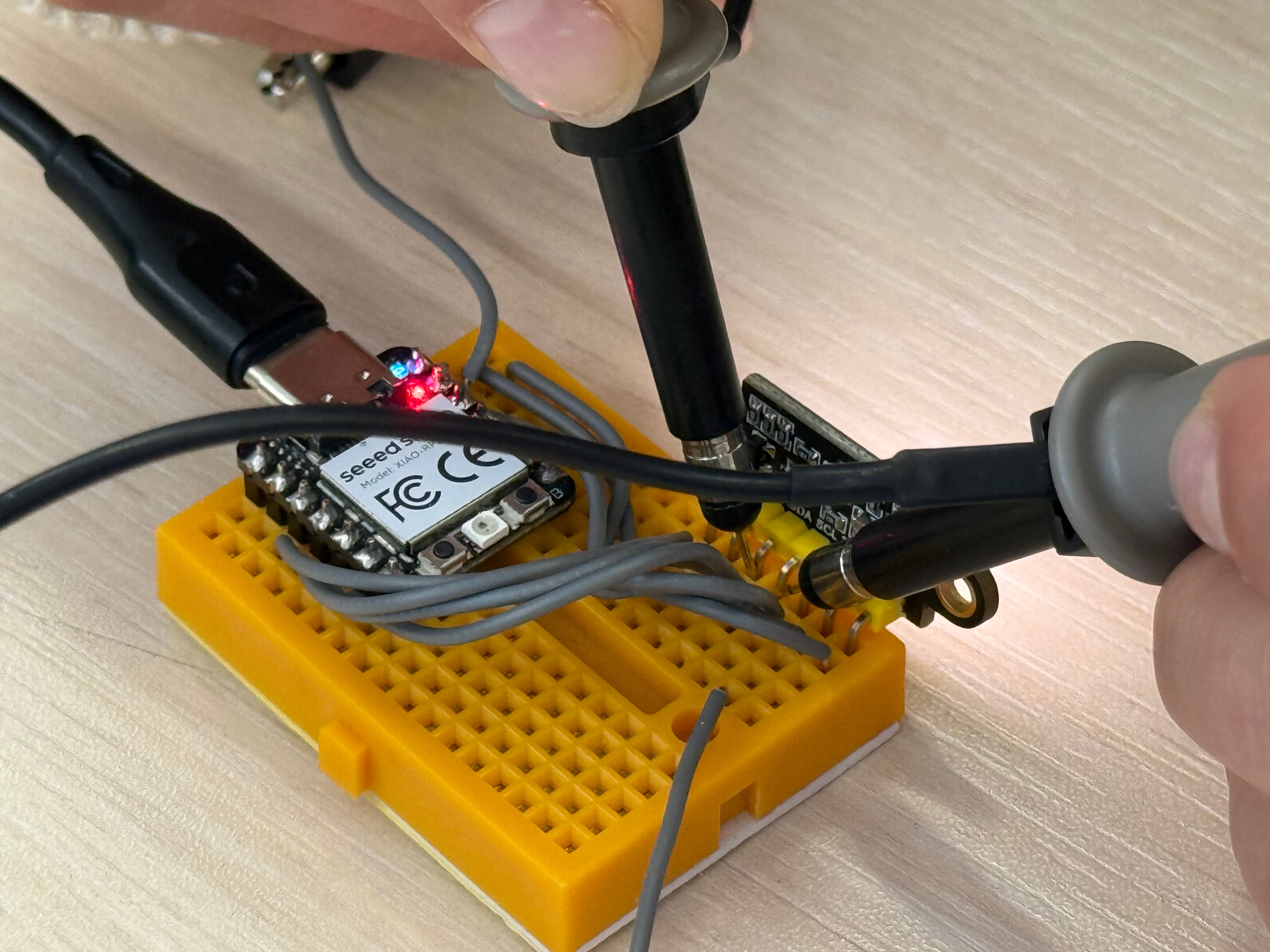
For our second experiment we connected a TCS34725 colour sensor to the Seeed XIAO RP2040 and probed the I2C communication lines (SDA and SCL) with the oscilloscope to see what digital communication looks like at signal level.

The Setup

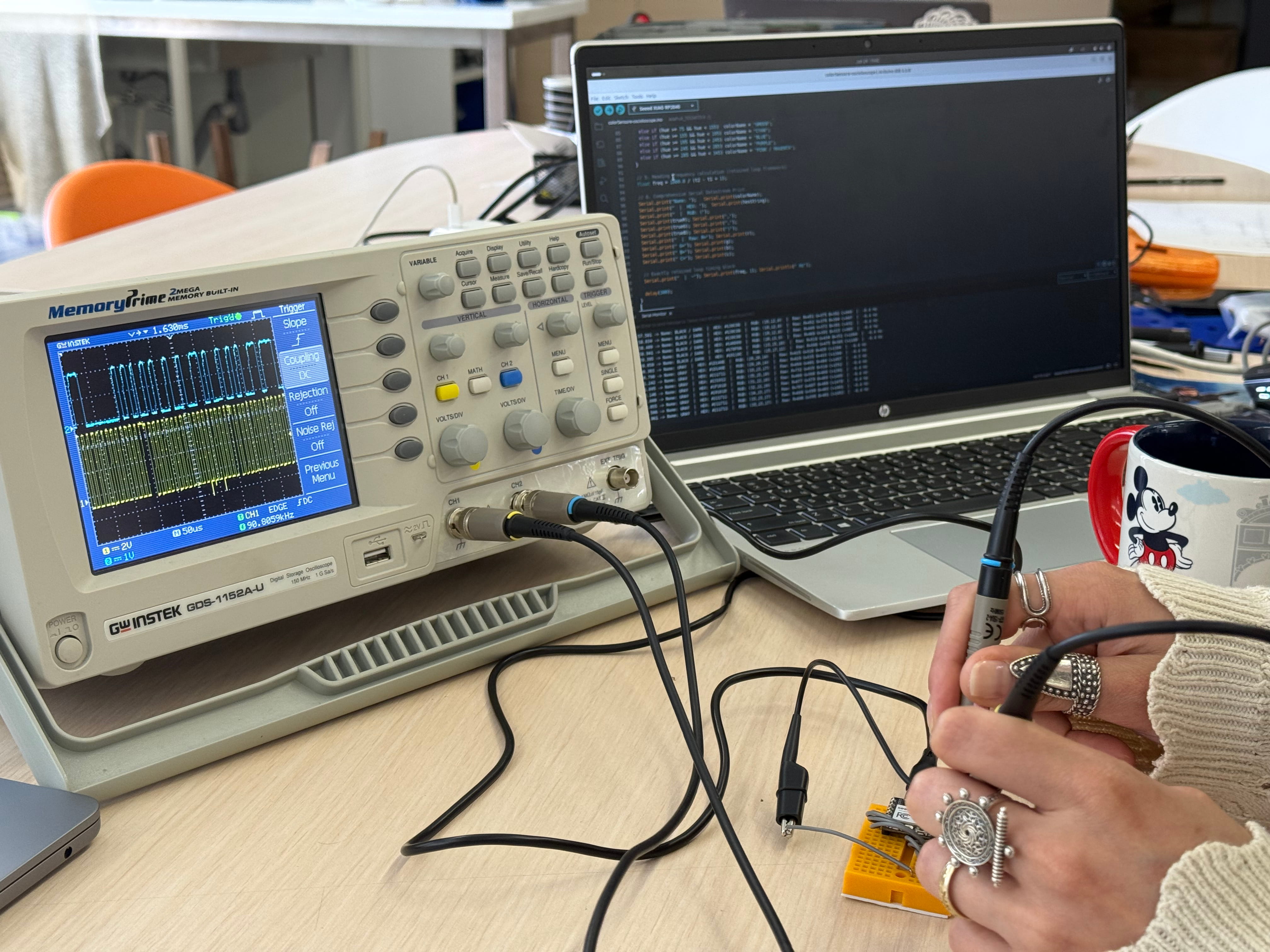
The TCS34725 communicates over I2C — two wires: SDA (data) and SCL (clock). We placed oscilloscope CH1 on SDA and CH2 on SCL, so we could watch both signals at the same time.

What the Oscilloscope Showed

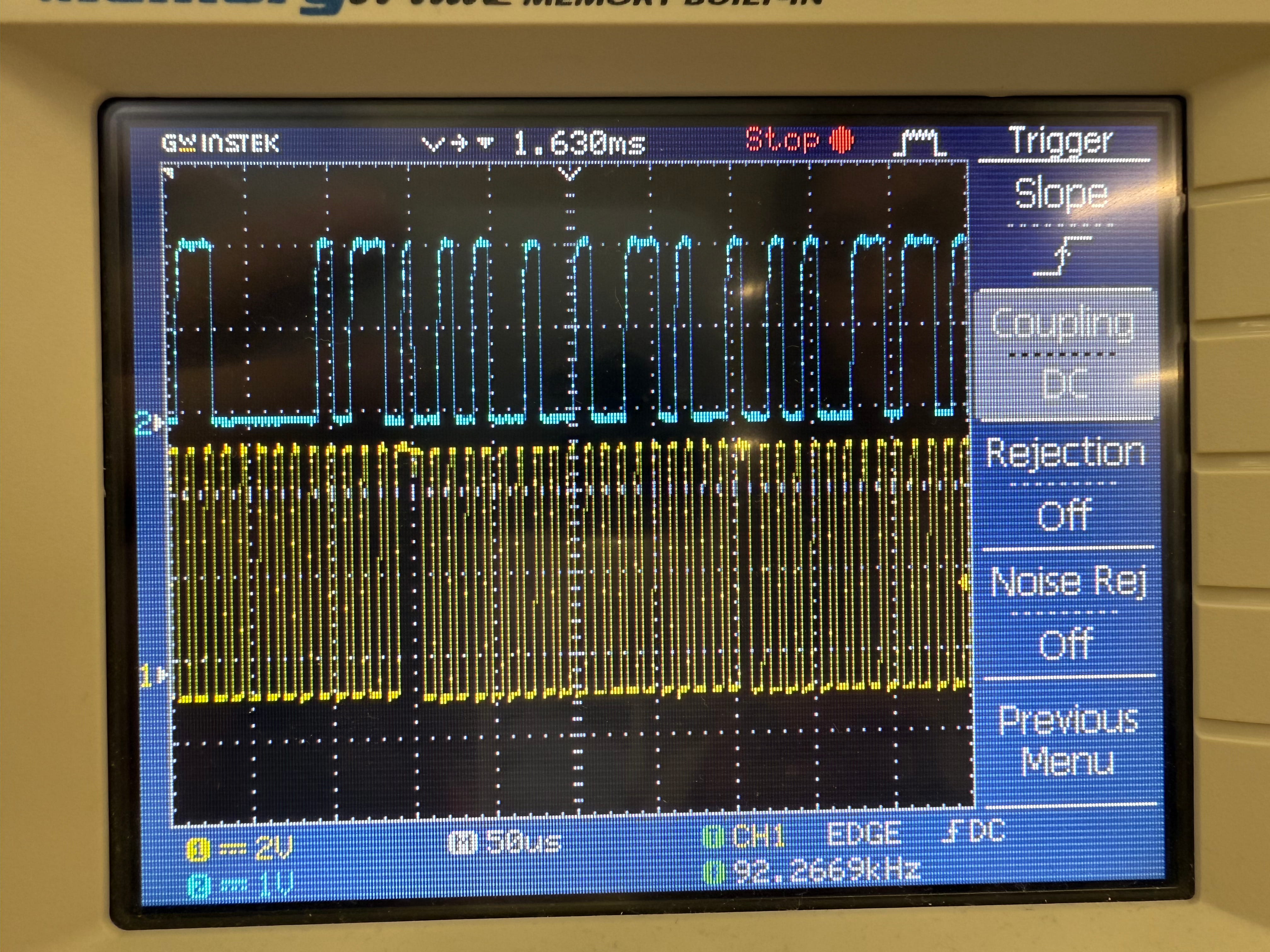
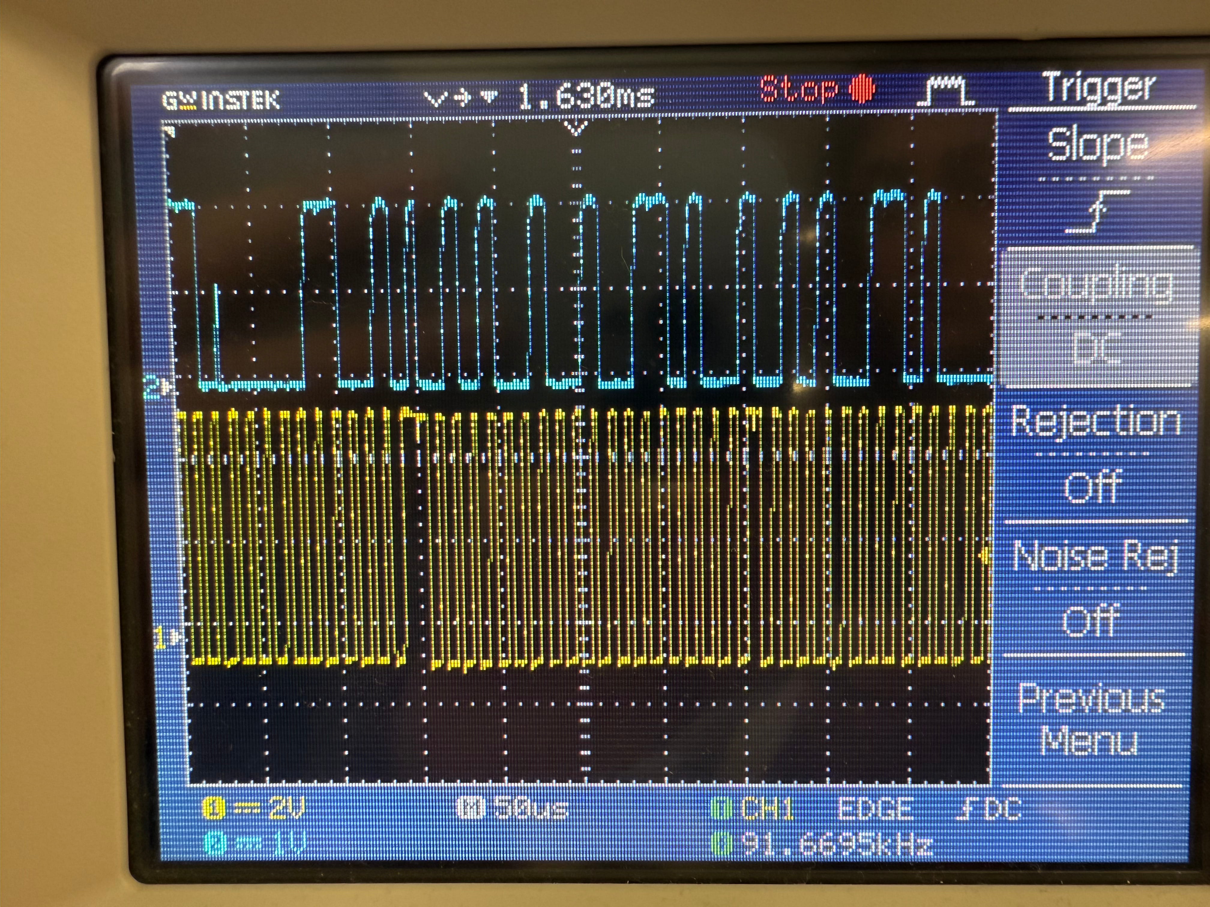
On the screen we could clearly see two channels: - CH1 (blue) — SDA: irregular pulses carrying the actual colour data — the pattern of highs and lows changes depending on what colour the sensor is reading - CH2 (yellow) — SCL: a steady, fast clock signal at around 92 kHz, ticking at the same rate regardless of colour

The oscilloscope measured the I2C clock at ~92.27 kHz — this is the RP2040 polling the sensor repeatedly as fast as it can. The time division was set to 50 µs/div.

The key observation: SCL is always regular and predictable, while SDA changes shape with every new reading — you can literally see different colours produce different bit patterns.

The Code

We wrote the firmware using Claude AI as a coding assistant, asking it to:

“Read TCS34725 colour sensor on RP2040, detect the colour name, output hex code and RGB values to Serial, show reading frequency.”

The resulting code uses HSV hue angle for colour classification (more accurate than comparing raw R/G/B values), plus white/black calibration constants so the sensor adapts to the ambient lighting conditions:

#include <Wire.h>
#include <Adafruit_TCS34725.h>

Adafruit_TCS34725 tcs = Adafruit_TCS34725(
  TCS34725_INTEGRATIONTIME_154MS,
  TCS34725_GAIN_4X
);

// Calibration — place white paper over sensor, copy raw values here
const uint16_t WHITE_R = 4500;
const uint16_t WHITE_G = 5200;
const uint16_t WHITE_B = 5500;

// Calibration — cover sensor completely, copy raw values here
const uint16_t BLACK_R = 120;
const uint16_t BLACK_G = 130;
const uint16_t BLACK_B = 120;

void setup() {
  Serial.begin(115200);
  Wire.begin();
  if (!tcs.begin()) {
    Serial.println("TCS34725 not found! Check wiring.");
    while (1);
  }
  Serial.println("Colour Scanner Online.");
}

void loop() {
  uint16_t r, g, b, c;
  tcs.getRawData(&r, &g, &b, &c);

  // Map raw sensor values to 0-255 using calibration range
  int trueR = map(constrain(r, BLACK_R, WHITE_R), BLACK_R, WHITE_R, 0, 255);
  int trueG = map(constrain(g, BLACK_G, WHITE_G), BLACK_G, WHITE_G, 0, 255);
  int trueB = map(constrain(b, BLACK_B, WHITE_B), BLACK_B, WHITE_B, 0, 255);

  // Output as HEX web colour code
  char hexString[8];
  sprintf(hexString, "#%02X%02X%02X", trueR, trueG, trueB);

  // Classify by hue angle
  // ... (full code available in repository)

  Serial.print("Name: ");  Serial.print(colorName);
  Serial.print("  |  HEX: "); Serial.print(hexString);
  Serial.print("  |  RGB: (");
  Serial.print(trueR); Serial.print(",");
  Serial.print(trueG); Serial.print(",");
  Serial.print(trueB); Serial.println(")");

  delay(300);
}

Serial Monitor Result

While probing with the oscilloscope, the Arduino Serial Monitor simultaneously showed the detected colour name, HEX code, and RGB values in real time — so we could cross-check what the I2C waveforms on the scope corresponded to in actual data.

What We Learned

Probing the I2C lines showed us that digital sensors don’t send a simple high/low signal — they send structured packets of data at a fixed clock rate. The SCL line is the heartbeat, and SDA carries the meaning. Watching the SDA pattern change as we moved the sensor over different colours made the link between physical reality and digital data very tangible.

---

Last update: July 6, 2026