Week 14 — Interface and application

TOOLS

Processing

Visual Programming

Bootstrap

Interface Design

Charts

Data Visualization

dat.GUI

Controls & Parameter Adjustment

This week I tried different tools to create interfaces and understand how they work together to develop an application. It was a new experience in my learning process because I didn’t know much about these tools, but I was surprised at all that can be achieved.

Tool 1 - Charts

One of the libraries that helped me understand how HTML works with different tools was Chart.js, which uses different types of charts and JavaScript plugins through the use of structured data for visual representation: bar charts, line charts, bubble charts, radar charts, etc...

A useful code example for understanding the structure of this library can be found in its tutorials. It provides a basic structure for creating a chart.js.

The canvas space is created using id="myChart".

1. The library we are using is included through src="https://cdn.jsdelivr.net/npm/chart.js" so that the browser can recognize it or can also be loaded from a local file using src="chart.umd.js".

2. const ctx = document.getElementById('myChart'); identifies the element where the chart will be drawn and new Chart(ctx, {}); allows you to create a chart.

3. The chart type is defined using type: 'bar', and the data is defined as follows:

data: {
  labels: ['Red', 'Blue', 'Yellow', 'Green', 'Purple', 'Orange'],
  datasets: [{
    label: '# of Votes',
    data: [12, 19, 3, 5, 2, 3],
    borderWidth: 1
  }]
},

labels contains the categories that will appear in the chart, and datasets contains the dataset.

The options property defines the behavior or appearance of the chart:

options: {
  scales: {
    y: {
      beginAtZero: true
    }
  }
}

You can also see that some of the basic parts of the code use JavaScript logic, similar to how it is used to modify or add interactive components to a page like this one.

<div>
  <canvas id="myChart"></canvas>
</div>

<script src="https://cdn.jsdelivr.net/npm/chart.js"></script>

<script>
  const ctx = document.getElementById('myChart');

  new Chart(ctx, {
    type: 'bar',
    data: {
      labels: ['Red', 'Blue', 'Yellow', 'Green', 'Purple', 'Orange'],
      datasets: [{
        label: '# of Votes',
        data: [12, 19, 3, 5, 2, 3],
        borderWidth: 1
      }]
    },
    options: {
      scales: {
        y: {
          beginAtZero: true
        }
      }
    }
  });
</script>.

After understanding the basic syntax of the code, we now try some examples we found.

The structure for these examples begins with the initial HTML tags and settings so that the browser can interpret the document and display the page.

1. <!DOCTYPE html>: Tells the browser that the document uses HTML5.

2. <html lang="en">: Indicates the language of the page.

3. <head>: Contains the initial configuration of the page.

4. <meta name="viewport" content="width=device-width, initial-scale=1.0">: Adjusts the page to the width of the device’s screen.

5. <title>Chart.js</title>: Sets the title that appears in the browser tab.

6. <script src="https://cdn.jsdelivr.net/npm/chart.js"></script>: Loads the Chart.js library.

<!DOCTYPE html>
<html lang="en">
<head>
  <meta name="viewport" content="width=device-width, initial-scale=1.0">
  <title>Chart.js</title>
  <script src="https://cdn.jsdelivr.net/npm/chart.js"></script>

Cascading Style Sheets (CSS)

<style>

  body {
    font-family: Arial, sans-serif;
    margin: 30px;
    background: #f5f5f5;
  }

  .charts-grid {
    display: grid;
    grid-template-columns: repeat(2, minmax(0, 1fr));
    gap: 24px;
  }

  .chart-container {
    background: white;
    padding: 20px;
    border-radius: 10px;
    min-width: 0;
    box-sizing: border-box;
  }

  .chart-area {
    height: 400px;
    position: relative;
  }

  button {
    padding: 12px 24px;
    margin-bottom: 30px;
    cursor: pointer;
  }

  @media (max-width: 800px) {

    .charts-grid {
      grid-template-columns: 1fr;
    }

  }

</style>

</head>

In this case, I created a button to make the data random and thus visualize the interaction of the charts, as well as establish their distribution and the order in which each one will appear.

<body>

  <button id="randomizeButton" type="button">
    Random
  </button>

  <div class="charts-grid">

    <div class="chart-container">

      <h2>Bar Chart</h2>

      <div class="chart-area">
        <canvas id="barChart"></canvas>
      </div>

    </div>

    <div class="chart-container">

      <h2>Line Chart</h2>

      <div class="chart-area">
        <canvas id="lineChart"></canvas>
      </div>

    </div>

    <div class="chart-container">

      <h2>Bubble Chart</h2>

      <div class="chart-area">
        <canvas id="bubbleChart"></canvas>
      </div>

    </div>

    <div class="chart-container">

      <h2>Radar Chart</h2>

      <div class="chart-area">
        <canvas id="radarChart"></canvas>
      </div>

    </div>

  </div>

  <script>

The global configuration of the data.

const DATA_COUNT = 7;

const labels = [
  'January',
  'February',
  'March',
  'April',
  'May',
  'June',
  'July'
];

const colors = [
  'rgb(255, 99, 132)',
  'rgb(54, 162, 235)',
  'rgb(75, 192, 192)'
];

function randomNumber(min, max) {

  return Math.floor(
    Math.random() * (max - min + 1)
  ) + min;

}

It's a bit funny here because each type of chart needs different data, so I declared a function that generates an array of values according to the type of chart.

function generateValues(type) {

  return Array.from(
    { length: DATA_COUNT },
    () => {

      if (type === 'bar') {

        const first = randomNumber(-100, 100);

        const second = randomNumber(-100, 100);

        return [
          Math.min(first, second),
          Math.max(first, second)
        ];

      }

      if (type === 'bubble') {

        return {
          x: randomNumber(0, 100),
          y: randomNumber(0, 100),
          r: randomNumber(5, 15)
        };

      }

      if (type === 'scatter') {

        return {
          x: randomNumber(0, 100),
          y: randomNumber(0, 100)
        };

      }

      if (type === 'radar') {

        return Math.random() < 0.2
          ? null
          : randomNumber(0, 100);

      }

      return randomNumber(-100, 100);

    }
  );

}

function generateData(type) {

  return {

    labels: labels,

    datasets: colors.map((color, index) => ({

      label: 'Dataset ' + (index + 1),

      data: generateValues(type),

      borderColor: color,

      backgroundColor: color.replace(
        'rgb(',
        'rgba('
      ).replace(
        ')',
        ', 0.4)'
      ),

      pointBackgroundColor: color,

      spanGaps: false

    }))

  };

}

We declare the creation of the charts.

const allCharts = [];

function createExample(canvasId, buildConfig) {

  const data = {
    labels: labels,
    datasets: []
  };

  const config = buildConfig(data);

  const generatedData = generateData(
    config.type
  );

  data.labels = generatedData.labels;

  data.datasets = generatedData.datasets;

  config.options = config.options || {};

  config.options.maintainAspectRatio = false;

  config.options.animation = {
    duration: 2000,
    easing: 'easeInOutQuart'
  };

  const chart = new Chart(
    document.getElementById(canvasId),
    config
  );

  allCharts.push(chart);

  return chart;

}

Finally, I pasted the examples from the tutorials to keep the configuration of each one.

createExample('barChart', (data) => {

  const config = {
    type: 'bar',
    data: data,
    options: {
      responsive: true,
      plugins: {
        legend: {
          position: 'top',
        },
        title: {
          display: true,
          text: 'Chart.js Floating Bar Chart'
        }
      }
    }
  };

  return config;

});


createExample('lineChart', (data) => {

  const config = {
    type: 'line',
    data: data,
    options: {
      responsive: true,
      plugins: {
        title: {
          display: true,
          text: 'Chart.js Line Chart'
        },
      },
      interaction: {
        mode: 'index',
        intersect: false
      },
      scales: {
        x: {
          display: true,
          title: {
            display: true,
            text: 'Month'
          }
        },
        y: {
          display: true,
          title: {
            display: true,
            text: 'Value'
          }
        }
      }
    },
  };

  return config;

});


createExample('bubbleChart', (data) => {

  const config = {
    type: 'bubble',
    data: data,
    options: {
      responsive: true,
      plugins: {
        legend: {
          position: 'top',
        },
        title: {
          display: true,
          text: 'Chart.js Bubble Chart'
        }
      }
    },
  };

  return config;

});


createExample('radarChart', (data) => {

  const config = {
    type: 'radar',
    data: data,
    options: {
      responsive: true,
      plugins: {
        title: {
          display: true,
          text: 'Chart.js Radar Skip Points Chart'
        }
      }
    },
  };

  return config;

});

To finish the code, I declared the action that generates new data for the four charts and connected the button to make it work.

const actions = [

  {
    name: 'Randomize',

    handler() {

      allCharts.forEach(chart => {

        chart.data.datasets.forEach(dataset => {

          dataset.data = generateValues(
            chart.config.type
          );

        });

        chart.update();

      });

    }

  }

];


document
  .getElementById('randomizeButton')
  .addEventListener('click', function() {

    actions[0].handler();

  });


</script>

</body>

</html>

Tool 2 - Processing

Another of the tools we use to have options for the final project is Processing that serves for graphics programming. I loved it for the practicality of its interface to render the codes, when testing many tools we had to look for codes from the community on the net to create our codes but adapted to our approach because here it changes the syntax a little for JAVA instead of JavaScript.

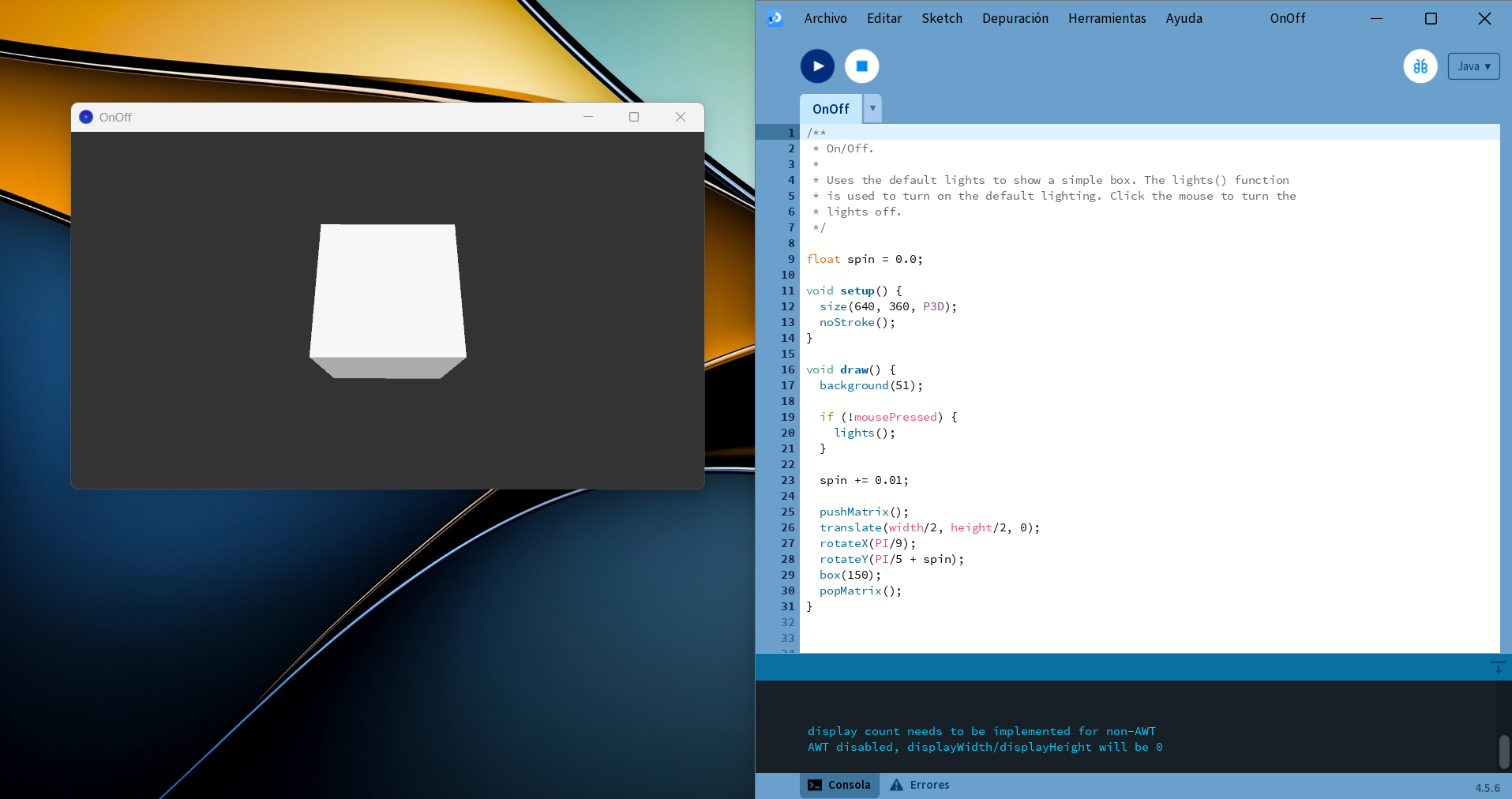
The examples use resources that the Processing documentation itself provides as a reference to understand the syntax.

Pointillism

float pointillize = map(mouseX, 0, width, smallPoint, largePoint);
color pix = img.get(x, y);

Ellipse
```
ellipse(224, 184, 220, 220);
```

Images and Pixels

float r = red(img.pixels[loc]);
float g = green(img.pixels[loc]);
float b = blue(img.pixels[loc]);

Random
```
float r = random(255);
stroke(r);
```

Load Image

PImage img;
img = loadImage("shells.jpg");
image(img, 0, 0);

Primitives 3D

translate(130, height/2, 0);
rotateY(1.25);
box(100);

Brownian Motion

ax[num-1] += random(-range, range);
ay[num-1] += random(-range, range);

Objects

Car myCar;

void setup() {
  myCar = new Car();
}

Line

size(400, 400);
line(120, 80, 340, 300);

Letters

char letter = char(counter);
text(letter, x, y);

Iteration

for (int i = 0; i < num; i++) {
  rect(405, y, 30, 10);
  y += 20;
}

Conditionals

if ((i % 20) == 0) {
  stroke(255);
  line(i, 80, i, height/2);
} else {
  stroke(153);
  line(i, 20, i, 180);
}

Sine Wave

void draw() {
  background(0);
  calcWave();
  renderWave();
}

Rectangles

size(400, 400);
rect(120, 80, 220, 220);

Keyboard Functions
```
void keyPressed()
```

Download File

Tool 3 - Bootstrap + p5.js + dat.GUI:

Bootsrap

The syntax of this file uses the same logic for creating a page that we used with Chart.js, but this time we added a line of code that loads Bootstrap from a CDN, allowing us to use its classes without having to write all the styles from scratch.

<link
  rel="stylesheet"
  href="https://cdn.jsdelivr.net/npm/bootstrap@5.3.3/dist/css/bootstrap.min.css"
>
</head>

1. The main container uses the available width and adds horizontal and vertical space, while the body of the page has a light background.

<body class="bg-light">
  <main class="container-fluid px-4 py-4">
  </main>
</body>

2. A row is created where each column occupies 6 of the 12 available columns starting at the medium screen size. Separation between the columns and space below the row are also added.

<div class="row g-3 mb-4">
  <div class="col-md-6">Heart Rate</div>
  <div class="col-md-6">Signal Status</div>
</div>

3. A card containing the information is created without a border, with a light shadow and a height of 100% relative to its container.

<div class="card border-0 shadow-sm h-100">
  <div class="card-body">
    <p class="text-secondary mb-2">Heart Rate</p>
  </div>
</div>

4. The value and unit are placed next to each other, aligned at the bottom and with space between them. The value is highlighted using a large, bold text size.

<div class="d-flex align-items-end gap-2">
  <span class="display-4 fw-bold">--</span>
  <span class="text-secondary mb-2">BPM</span>
</div>

5. Labels are created to display statuses, and different colors are used to distinguish them.

<span class="badge text-bg-secondary">No data</span>
<span class="badge text-bg-light border text-secondary">IDLE</span>
<span class="badge text-bg-danger">Offline</span>

6. The layout of the interface is adjusted according to the screen size.

<div class="row g-4 align-items-stretch">
  <div class="col-12 col-xl-3">dat.GUI</div>
  <div class="col-12 col-xl-6">ECG Signal</div>
  <div class="col-12 col-xl-3">Device Status / Connection</div>
</div>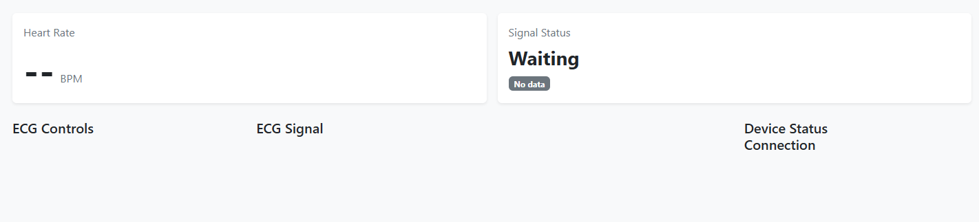

7. The content is centered horizontally and vertically. A border with rounded corners is also added, and light or dark backgrounds are used.

<div
  class="border rounded bg-light d-flex justify-content-center align-items-center text-secondary text-center p-3"
  style="min-height: 350px;"
>
  ECG controls will appear here
</div>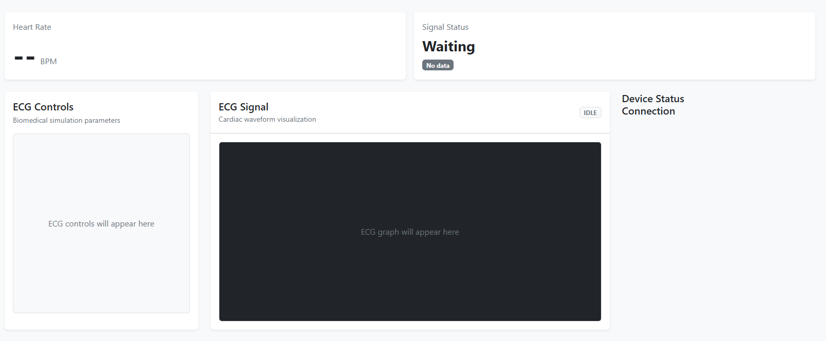

8. The cards are stacked with space between them. A card can grow if there is free height, and the elements can be placed at opposite ends of their container.

<div class="d-flex flex-column gap-4 h-100">
  <div class="card border-0 shadow-sm">Device Status</div>
  <div class="card border-0 shadow-sm flex-grow-1">Connection</div>
</div>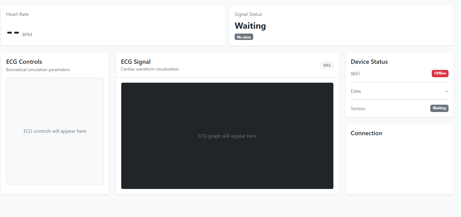

9. The label is linked to the input field, styles are applied to both elements, and a sample IP address is displayed within the field.

<label for="deviceIP" class="form-label">Device IP</label>
<input id="deviceIP" type="text" class="form-control mb-3" placeholder="192.168.1.100">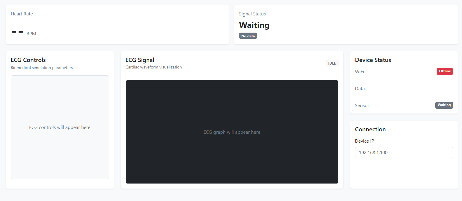

10. The buttons are placed in a column with space between them, and a base style is applied to them.

<div class="d-grid gap-2">
  <button type="button" class="btn btn-primary">Connect</button>
  <button type="button" class="btn btn-outline-secondary">Disconnect</button>
  <button type="button" class="btn btn-outline-success">Start Demo</button>
</div>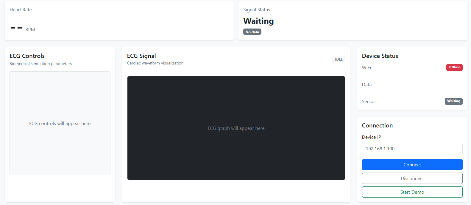

p5.js

1. We use the same logic to create an HTML structure for the code, but in this case we are going to use p5.js by loading the library.

<script src="https://cdn.jsdelivr.net/npm/p5@1.11.1/lib/p5.min.js"></script>

2. Some CSS settings for the page structure.

#ecgCanvas {
  width: 100%;
  max-width: 900px;
  height: 350px;
  margin: 0 auto;
  border-radius: 8px;
  overflow: hidden;
}

3. The container for the graph.

<div id="ecgCanvas"></div>

4. We declare the variables; timeOffset starts at zero and will increase over time.

let timeOffset = 0;

const heartRate = 60;
const paperSpeed = 25;
const gain = 10;

5. We start declaring the canvas functions with setup().

function setup() {

  const box =
    document.getElementById("ecgCanvas");

  const canvas =
    createCanvas(
      Math.max(300, box.clientWidth),
      350
    );

  canvas.parent("ecgCanvas");
}

6. Now we add a function for the signal animation so that, in each cycle, the canvas is cleared, the grid and the signal are drawn, and the time is updated.

function draw() {

  background(
    15,
    18,
    22
  );

  drawECGGrid();
  drawECGSignal();

  timeOffset +=
    deltaTime / 1000;
}

7. Having declared the animation, we proceed to draw the ECG line by taking the signal values and converting each point into a position within the canvas.

function drawECGSignal() {

  const pixelsPerMM = 5;

  const pixelsPerSecond =
    paperSpeed * pixelsPerMM;

  const pixelsPerMV =
    gain * pixelsPerMM;

  const beatPeriod =
    60 / heartRate;

  stroke(
    0,
    255,
    120
  );

  strokeWeight(2);
  noFill();

  beginShape();

  for (
    let x = 0;
    x < width;
    x++
  ) {

    const time =
      x / pixelsPerSecond +
      timeOffset;

    const beatTime =
      time % beatPeriod;

    const voltage =
      ecgSignal(
        beatTime,
        beatPeriod
      );

    const y =
      height / 2 -
      voltage *
      pixelsPerMV;

    vertex(
      x,
      y
    );
  }

  endShape();
}

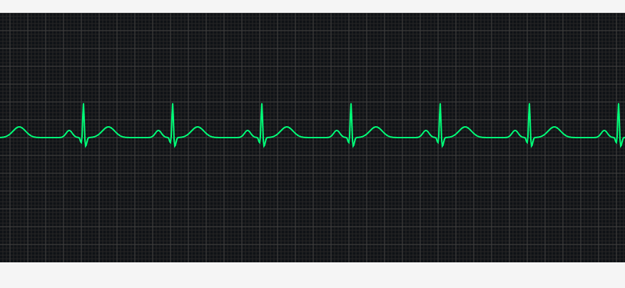
8. The creation of the P-QRS-T shape.

function ecgSignal(
  time,
  period
) {

  let voltage = 0;

  const rCenter =
    min(
      0.35,
      period * 0.42
    );

  const pCenter =
    rCenter - 0.16;

  const qCenter =
    rCenter - 0.025;

  const sCenter =
    rCenter + 0.025;

  const tCenter =
    min(
      rCenter + 0.28,
      period - 0.08
    );

  voltage +=
    gaussian(
      time,
      pCenter,
      0.035,
      0.20
    );

  voltage +=
    gaussian(
      time,
      qCenter,
      0.010,
      -0.15
    );

  voltage +=
    gaussian(
      time,
      rCenter,
      0.008,
      1.00
    );

  voltage +=
    gaussian(
      time,
      sCenter,
      0.012,
      -0.25
    );

  voltage +=
    gaussian(
      time,
      tCenter,
      0.070,
      0.30
    );

  return voltage;
}

9. The shape of each wave.

function gaussian(
  x,
  center,
  width,
  amplitude
) {

  return
    amplitude *
    exp(
      -pow(
        x -
        center,
        2
      ) /
      (
        2 *
        pow(
          width,
          2
        )
      )
    );
}

10. Finally, we adapt the canvas to the size of the window.

function windowResized() {

  const box =
    document.getElementById("ecgCanvas");

  resizeCanvas(
    Math.max(
      300,
      box.clientWidth
    ),
    350
  );
}

dat.GUI

We will use this library for the interface because we will add a demo mode to simulate different ECG waveforms.

<script src="https://cdn.jsdelivr.net/npm/dat.gui@0.7.9/build/dat.gui.min.js"></script>

1. To return all the parameters to their initial values and update the interface controls, a reset function is created.

reset: function() {

  settings.heartRate = 60;

  settings.pAmplitude = 0.20;
  settings.prInterval = 160;

  settings.qrsDuration = 90;
  settings.rAmplitude = 1.00;

  settings.stLevel = 0.00;

  settings.tAmplitude = 0.30;
  settings.qtInterval = 380;

  settings.gain = 10;
  settings.paperSpeed = 25;

  settings.baselineWander = 0;
  settings.noiseLevel = 0;

  settings.mainsFrequency = "Off";
  settings.mainsAmplitude = 0;

  settings.lineWidth = 2;
  settings.signalColor = "#00ff78";

  settings.showGrid = true;
  settings.paused = false;

  gui.updateDisplay();
}

2. Next, the dat.GUI interface is created.

const gui =
  new dat.GUI();

3. Finally, the controls are organized into different folders; each folder contains the corresponding parameters with their minimum, maximum, and increment values.

const morphology =
  gui.addFolder("ECG Morphology");

morphology.add(
  settings,
  "heartRate",
  30,
  180,
  1
).name("Heart Rate (BPM)");

morphology.add(
  settings,
  "pAmplitude",
  0,
  0.5,
  0.01
).name("P Amplitude (mV)");

morphology.add(
  settings,
  "prInterval",
  80,
  300,
  1
).name("PR Interval (ms)");

morphology.add(
  settings,
  "qrsDuration",
  40,
  200,
  1
).name("QRS Duration (ms)");

morphology.add(
  settings,
  "rAmplitude",
  0.2,
  2.5,
  0.05
).name("R Amplitude (mV)");

morphology.add(
  settings,
  "stLevel",
  -0.5,
  0.5,
  0.01
).name("ST Level (mV)");

morphology.add(
  settings,
  "tAmplitude",
  -0.5,
  0.8,
  0.01
).name("T Amplitude (mV)");

morphology.add(
  settings,
  "qtInterval",
  250,
  600,
  1
).name("QT Interval (ms)");

morphology.open();


const acquisition =
  gui.addFolder("Acquisition");

acquisition.add(
  settings,
  "gain",
  [5, 10, 20]
).name("Gain (mm/mV)");

acquisition.add(
  settings,
  "paperSpeed",
  [25, 50]
).name("Speed (mm/s)");

acquisition.add(
  settings,
  "baselineWander",
  0,
  0.5,
  0.01
).name("Baseline Drift (mV)");

acquisition.add(
  settings,
  "noiseLevel",
  0,
  0.2,
  0.01
).name("Noise (mV)");

acquisition.add(
  settings,
  "mainsFrequency",
  [
    "Off",
    "50 Hz",
    "60 Hz"
  ]
).name("Power Line");

acquisition.add(
  settings,
  "mainsAmplitude",
  0,
  0.2,
  0.01
).name("Power Noise (mV)");


const display =
  gui.addFolder("Display");

display.add(
  settings,
  "lineWidth",
  1,
  6,
  1
).name("Trace Width");

display.addColor(
  settings,
  "signalColor"
).name("Trace Color");

display.add(
  settings,
  "showGrid"
).name("ECG Grid");

display.add(
  settings,
  "paused"
).name("Pause");

display.add(
  settings,
  "reset"
).name("Reset ECG");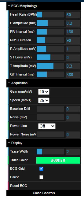

Integration

1. Bootstrap: Creates and organizes the visual structure of the interface.

<div class="row g-4 align-items-stretch" id="monitorRow">

  <div id="guiColumn" class="col-12 col-lg-4 col-xxl-3 d-none">

    <div id="guiCard" class="card border-0 shadow-sm">

      <div class="card-header bg-white py-3">

        <h5 class="mb-0">
          ECG Controls
        </h5>

      </div>

      <div id="guiPanel"></div>

    </div>

  </div>


  <div id="signalColumn" class="col-12 col-lg-8">

    <div id="ecgCard" class="card border-0 shadow-sm">

      <div class="card-body">

        <div
          id="ecgCanvas"
          class="border rounded bg-dark overflow-hidden">
        </div>

      </div>

    </div>

  </div>

</div>

2. p5.js: Draws and animates the ECG signal inside the canvas.

function setup() {

  const box =
    $('ecgCanvas');

  createCanvas(
    Math.max(
      1,
      box.clientWidth
    ),
    Math.max(
      1,
      box.clientHeight || 350
    )
  ).parent(
    'ecgCanvas'
  );

  createControls();

  resetConnectionUI();
}

3. dat.GUI: Generates the controls for the demo mode.

function createControls() {

  gui =
    new dat.GUI({
      autoPlace: false,
      width: 320
    });

  $('guiPanel').appendChild(
    gui.domElement
  );

  const morph =
    gui.addFolder(
      'ECG Morphology'
    );

  morph.add(
    settings,
    'heartRate',
    30,
    180,
    1
  ).name(
    'Heart Rate (BPM)'
  );

  const display =
    gui.addFolder(
      'Display'
    );

  display.addColor(
    settings,
    'signalColor'
  ).name(
    'Trace Color'
  );
}

4. WebSocket: Receives the data sent by the XIAO through the network connection.

function connectToDevice() {

  const input =
    $('deviceIP').value.trim();

  // Connection URL configuration

  const ws =
    new WebSocket(
      url
    );

  socket =
    ws;

  ws.onmessage =
    event => {

      const data =
        JSON.parse(
          event.data
        );

      if (
        data.type !== 'sample'
      )
        return;

      const ecg =
        Number(
          data.ecg
        );

      ecgSamples.push(
        ecg
      );
    };
}

5. JavaScript: Coordinates the interface logic and decides which signal mode is displayed.

function draw() {

  background(
    15,
    18,
    22
  );

  if (
    !demoMode &&
    !deviceMode
  ) {

    drawIdleSignal();
    return;
  }

  if (
    settings.showGrid
  )
    drawECGGrid();

  if (
    deviceMode
  ) {

    drawDeviceSignal();
    return;
  }

  drawECGSignal();

  if (
    !settings.paused
  )
    timeOffset +=
      deltaTime /
      1000;
}

Download File

Deployment

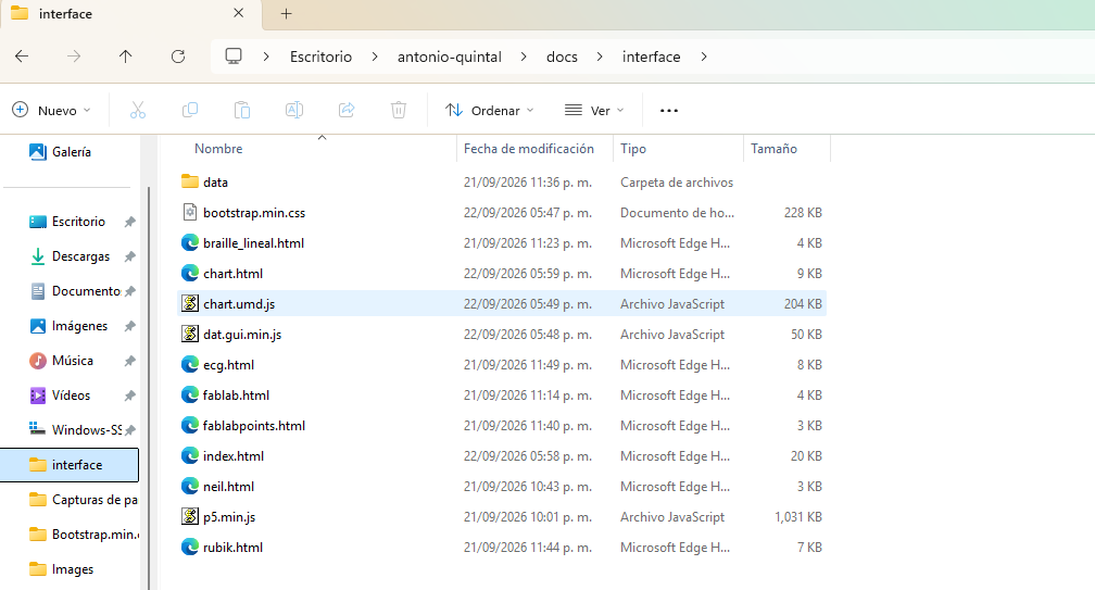
To integrate all my code and be able to view it within the assignment, I incorporated it into my MkDocs project using the same code, but now integrated as HTML files. I added the libraries locally so that the project would not depend on an external connection through a CDN, and I saved them inside my repository folder.