Development Logbook<
Introduction<
This development logbook regroups all the works that have been done during the Fab Academy which are related to my final project. Most of the time, the presented works were done for specific assignments. In that case, you will find pictures that summarized the work done and a link directing to the corresponding week. In the other case, the presented works were done during "break" times or between assignments. These works will be more detailed on this webpage. Enjoy your reading !
Week 6 : Electronic Design<
Week 8 : Electronic Production<
Week 9 : Input Devices<
Midterm Break : Testing the Idea<
Below you may find the work done during the midterm break. I decided it was time to test the concept behind my final project idea. Therefore I started by recalling how it is supposed to work theoretically and then developped a first prototype using the Open UC2 toolbox. At first I used the latter because it was already there in my lab but later I realised using this toolbox would be a good idea for system integration and for later uses of my project. You may find more informations in the Week 15 documentation.
Theory Summary<
General Principle<
A common way to measure particles density in aerosols, called liquid water content ("LWC"), is to use light absorbtion and scattering by either measuring how much light is transmitted through the aerosol depending on its LWC or directly how much light is scattered. If one even manage to measure the directions at which the light is scattered, they could obtain informations about particles sizes distribution.
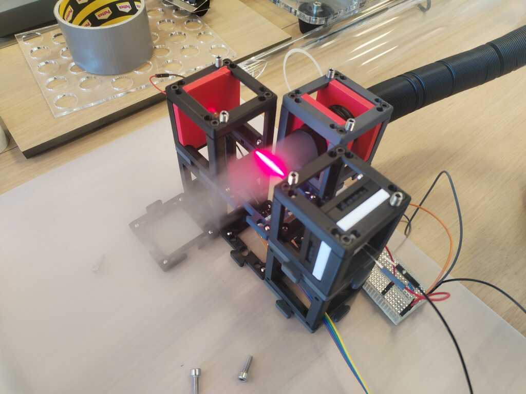
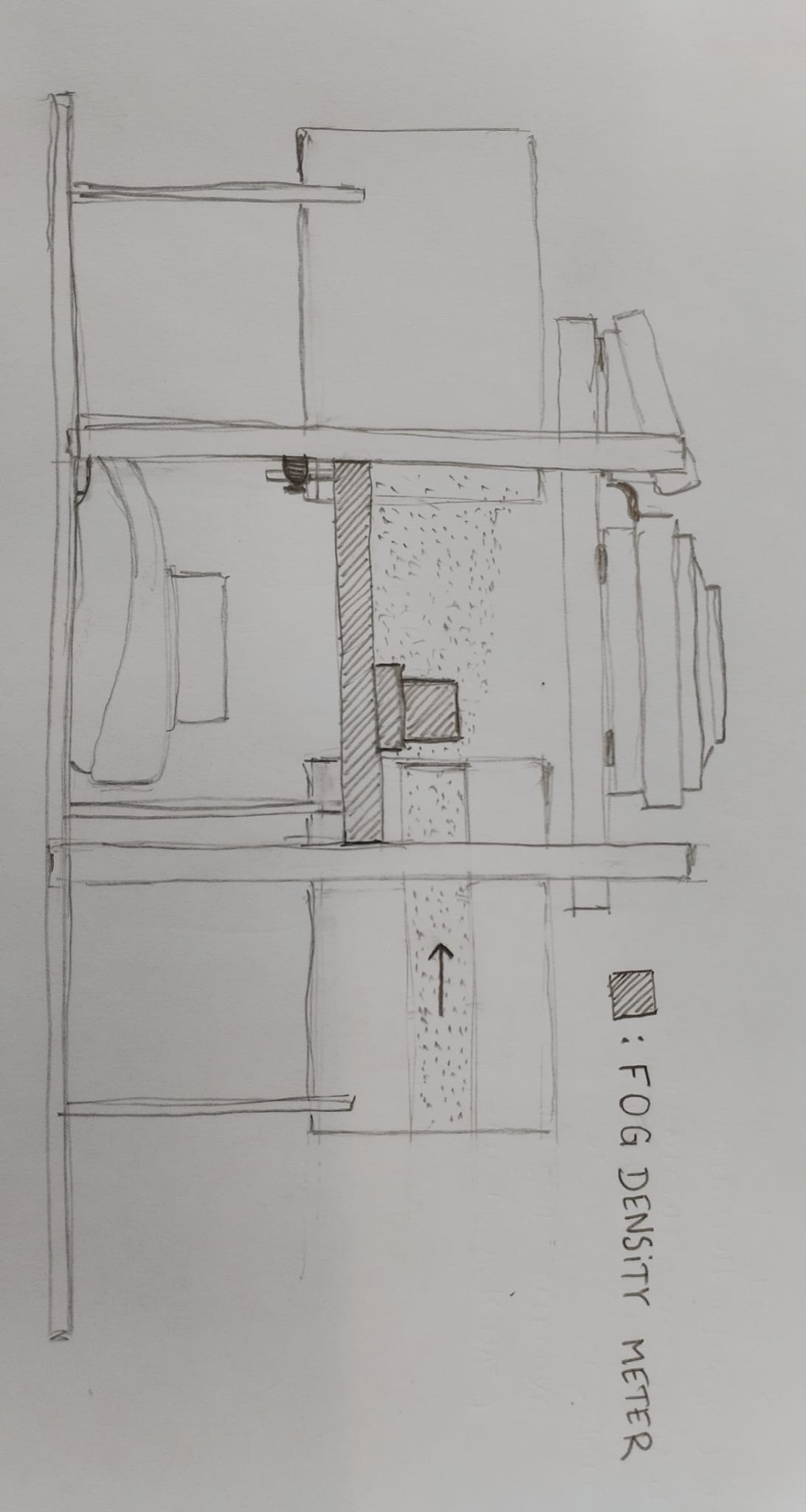
When light interracts with fog, there is a probability that it scatters on a droplet or is absorbed by the latter. By installing a laser going through the fog and a photosensor right in front of the laser, one could measure the light intensity diminution due to the presence of the fog.

Calibration<
Transmitted signal<
Let's consider a beam of light entering a fog sample. We define \(z\) as an axis parallel to the direction of the beam. According to Beer-Lambert's law, the transmitted light intensity \(L_{out}\) is given by :
where \(L_0\) is the emitted light intensity, \(\sigma\) is the cross section of the interaction light-droplet, \(n(z)\) is the number density of water droplets, \(l\) is the fog thickness. Therefore if the fog is homogeneous (which we will assume to begin), \(n\) is independent of \(z\) and the latter equation can be transformed as :
On the other side, liquid water content is defined as :
therefore, by combining both equations we get :
However the cross section \(\sigma\) is hard to determine hence we will have to calibrate our measurment with a known \(LWC\).
Let's not forget that our device will not directly give the light intensity \(L\) but a voltage. Indeed we will use a phototransistor that generates a current \(I\) proportionnal to the received light intensity :
where \(S_{ph}\) is the phototransistor's sensitivity. The phototransistor's collector is in series with a resistor \(R\) which is connected to the power source \(V_{CC}\) and the emitter is connected to the ground. The measured voltage is thus the one between the collector and the emitter, \(V_{CE}\) hence :
and, isolating \(L\) :
therefore :
where \(\alpha(r,\rho,\sigma)\) contains all the parameters we don't know hence it has to be determined by calibrating our device with a known \(LWC\).
Scattered signal<
Let's now reconsider a beam of light entering a fog sample however one measure the intensity of the scattered light at a certain angle \(\theta\), \(L_\theta\). The latter can be shown to be proportionnal to the droplets number density \(n\) and the scattering cross section \(\sigma_s\) :
using a similar argumen to the previous one, one can show that :
where \(\beta(r, \rho, \sigma_s, R, S_{ph})\) contains all the parameters we don't know hence it has to be determined by calibrating our device with a known \(LWC\).
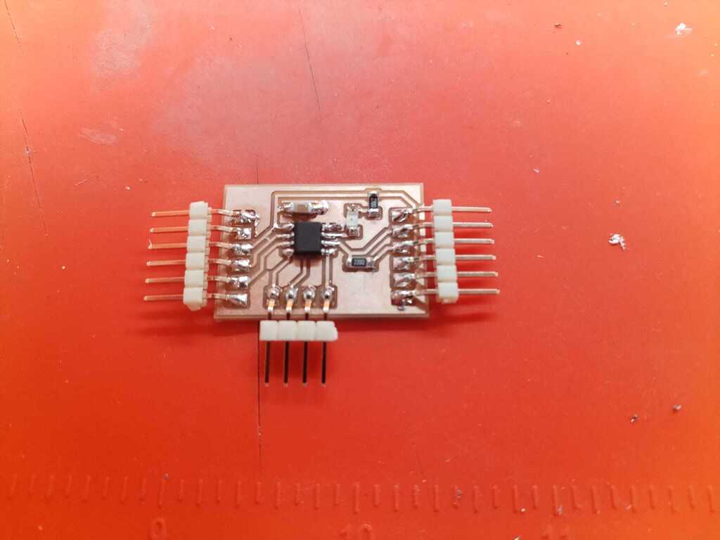
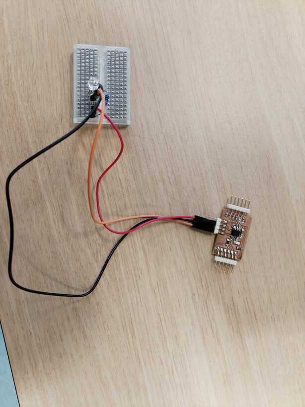
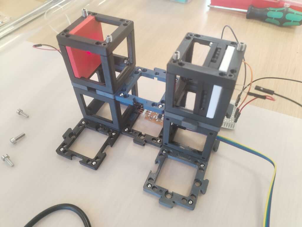
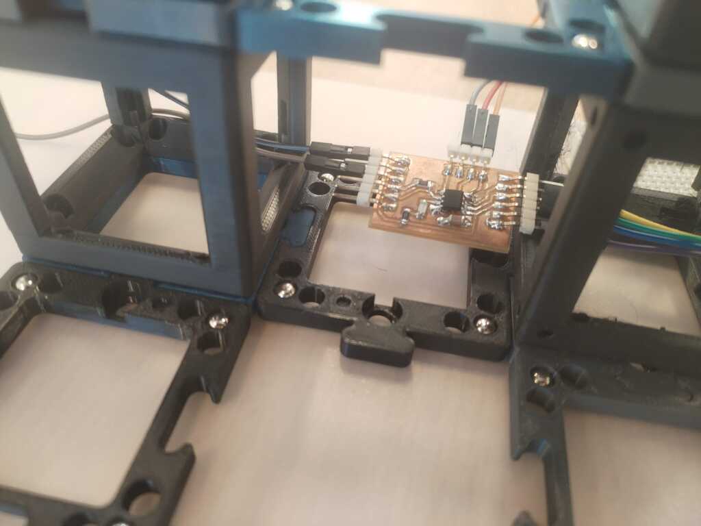
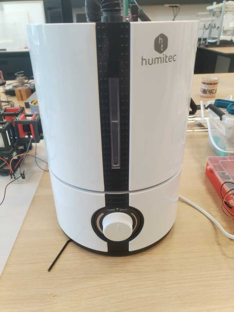
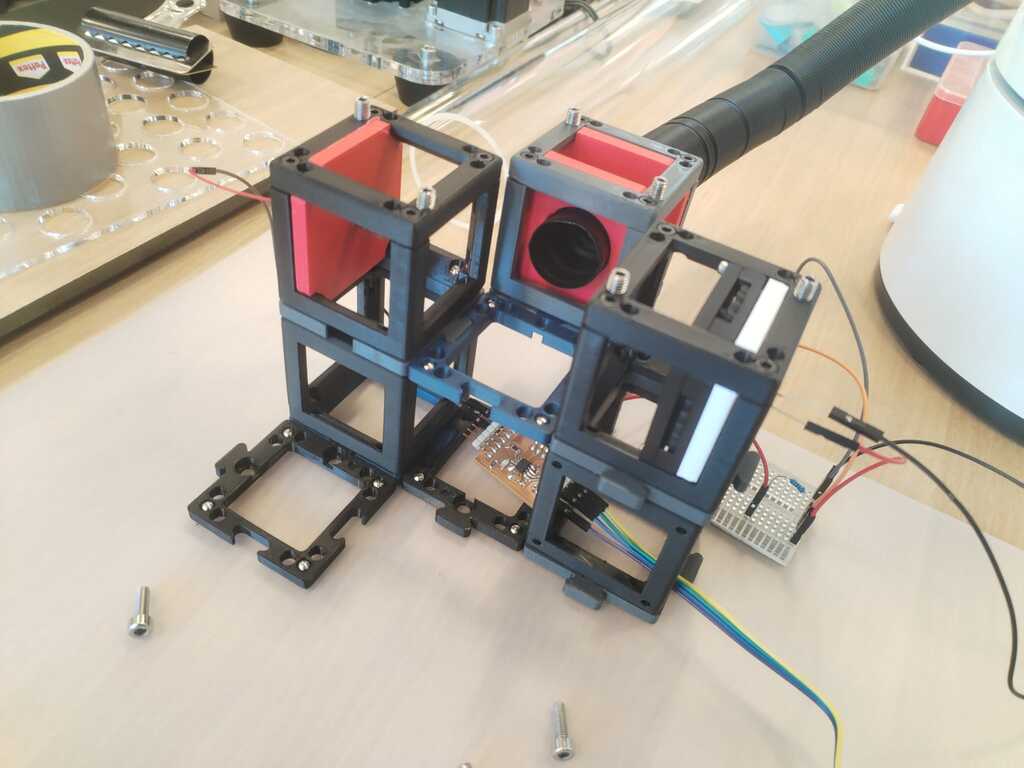
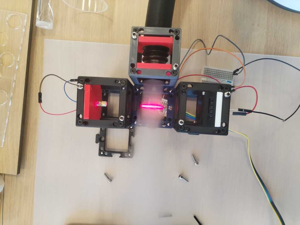
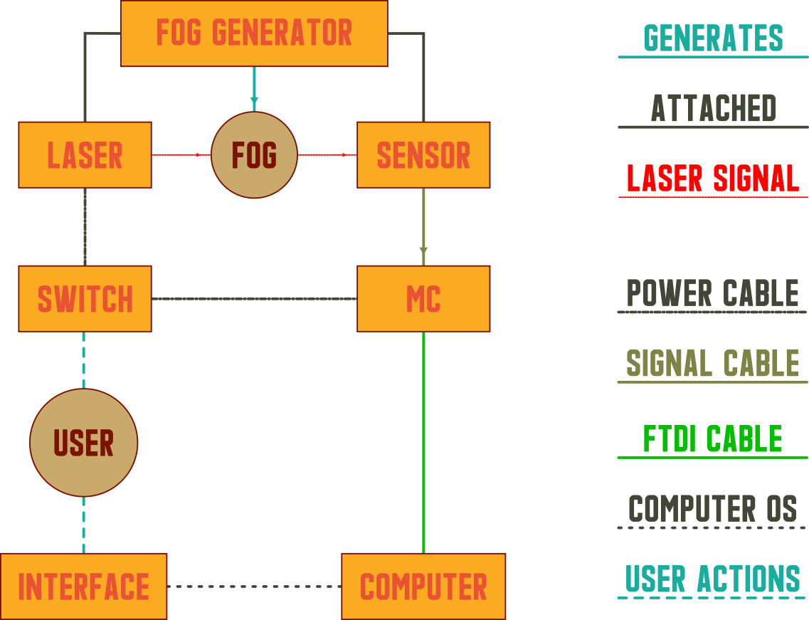
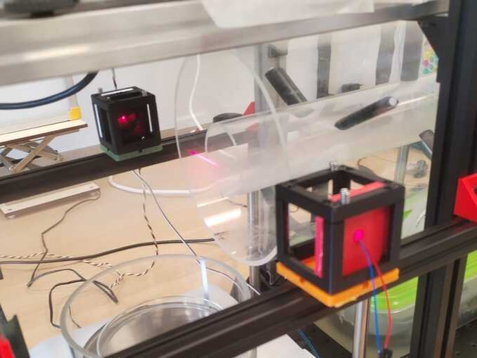
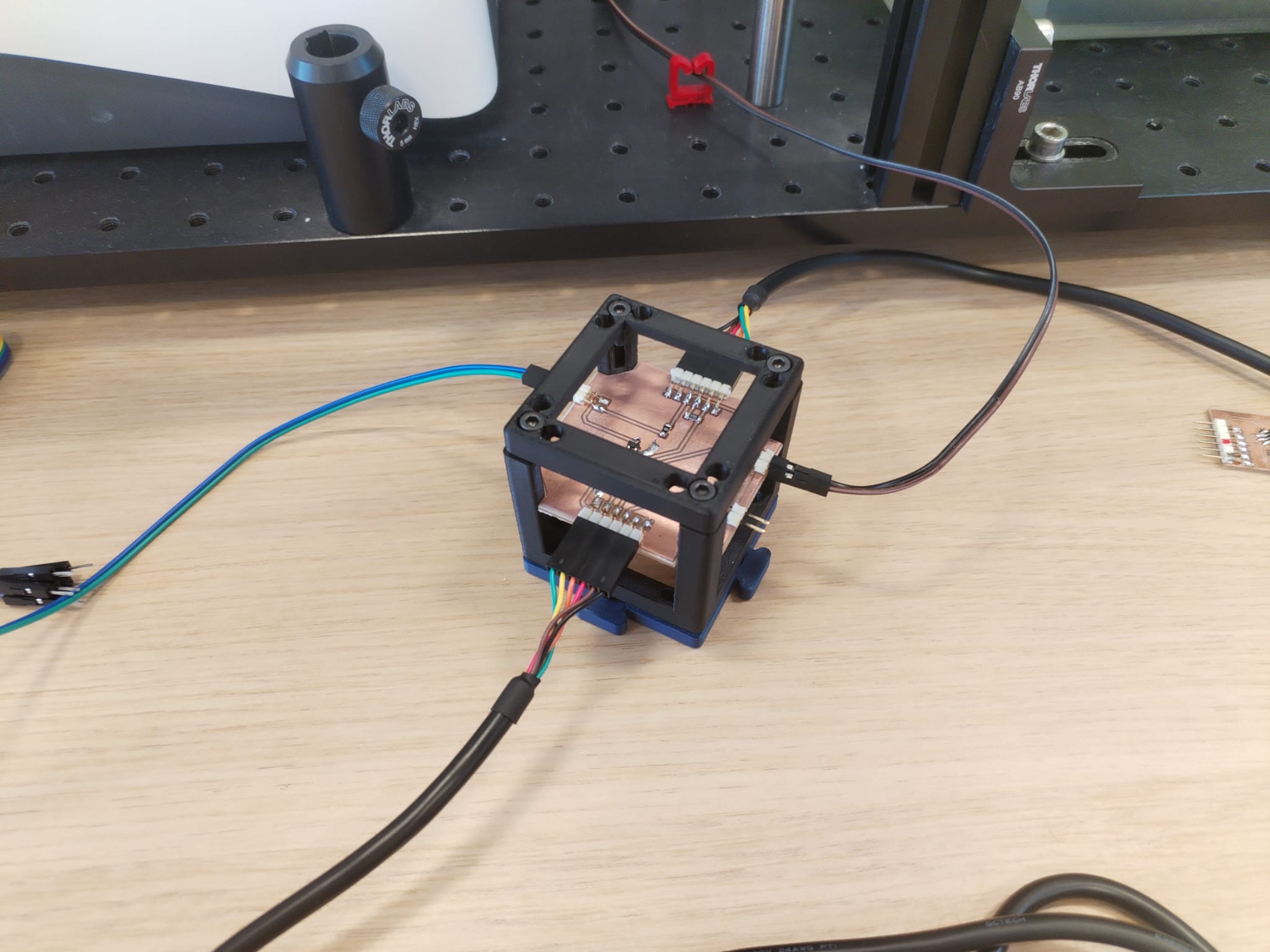
First Prototype Development<
I built a first prototype using the Open UC2 cubes and a commercial fog generator.
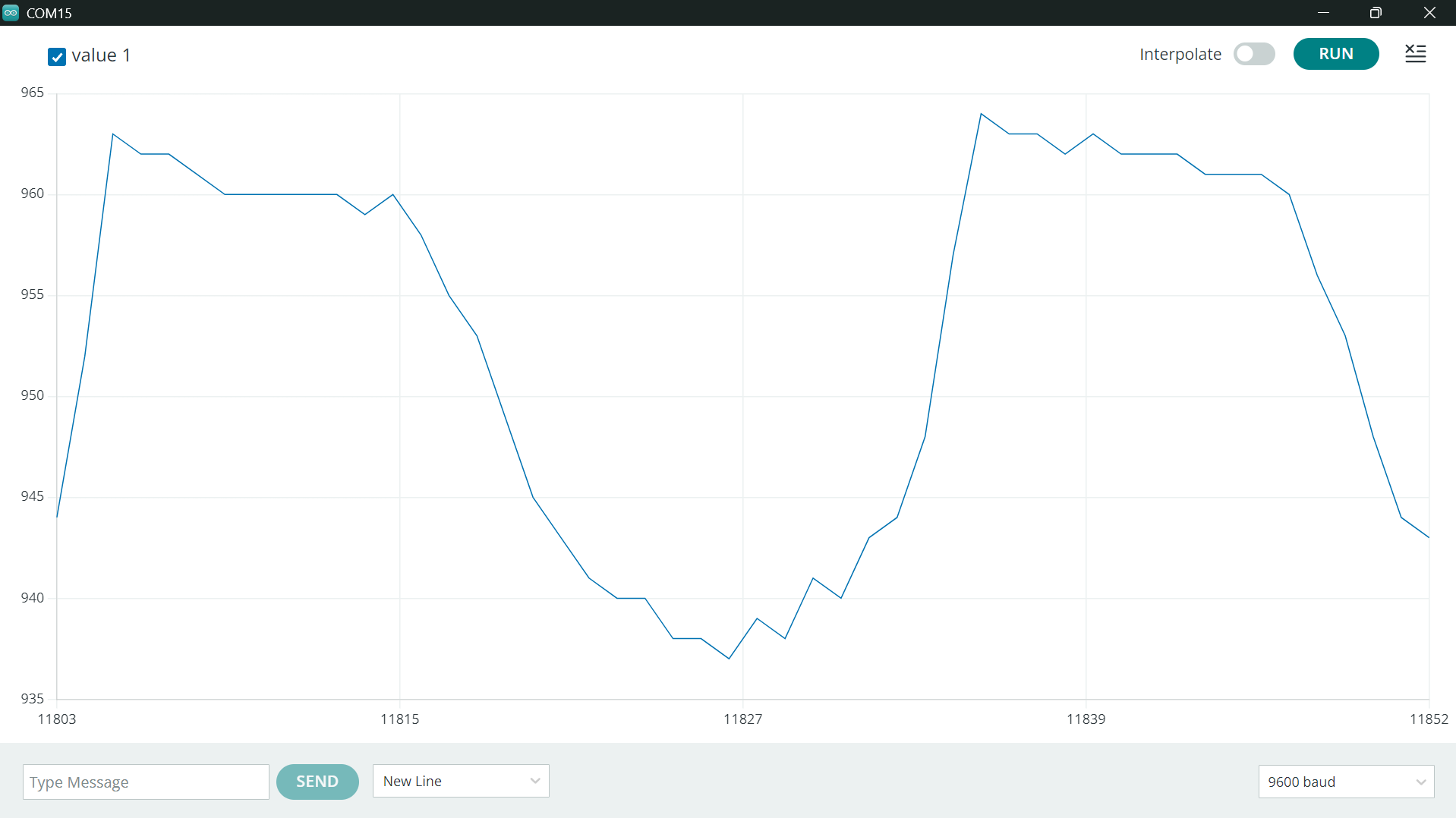
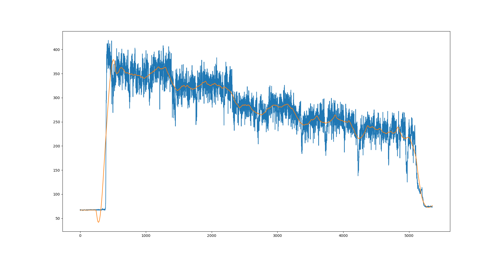
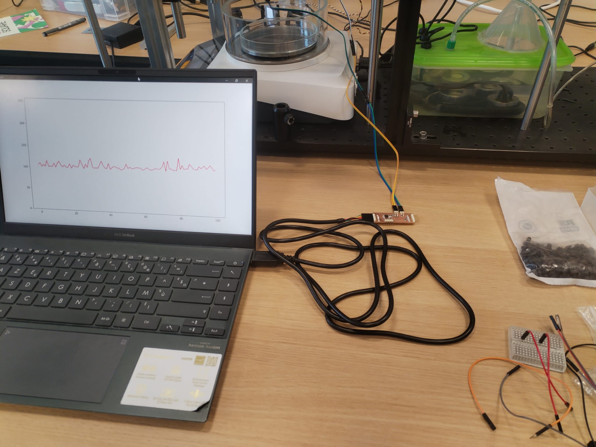
First look at data<
I accessed the data through the Arduino Interface. I waited a bit and then copied pasted the serial monitor content in a txt file. I then wrote a small python script to visualise and filter them. Below you may find the code and the plot result.
import pandas as pd
from scipy.signal import savgol_filter
import matplotlib.pyplot as plt

df = pd.read_csv("EXP-2.txt", sep=",",names=["Max", "Min","Data"])

signal = df.Data

window=301

smooth_signal = savgol_filter(signal, window_length=window, polyorder=3, deriv=0)

plt.plot(signal)
plt.plot(smooth_signal)

print(signal.size)
Week 14 : Interface<
Week 15 : System Integration<
Week 17 : Synchronous Detection<
Introduction<
During the seventeeth week's global review I was random picked to present my final project and my sixteenth week's assignment. After seeing my final project overview, Neil suggested that I look into synchronous detection and more specifically lock-in amplifier in order to use a LED instead of a laser.
Indeed, lasers may be hard to align with photosensors while LED are more diffused however in return, a sensed signal produced by a far LED is way weaker than laser's one. This can be a problem in noisy conditions hence one may use a technique called lock-in amplifier defined by Wikipedia as :
A lock-in amplifier is a type of amplifier that can extract a signal with a known carrier wave from an extremely noisy environment.
General lock-in amplifier relies on the orthogonality of sinusoidal functions however in its simplest form, which is the one we will use, it does not require understanding this kind of math. The simplest lock-in amplifier consists in performing fast repeated measurements while turning on and off the signal's source, then averaging over a few measurments and substracting the \(<OFF>\) average to the \(<ON>\) average. Let's explain why it works.
When the light source is on, the sensor measures :
where \(L\) is the usefull signal and \(B\) is the ambient noise.
When the light source is off, the sensor measures :
if a large number of measurments is made rapidly and the latter are averaged we get :
which then corresponds to the average of the usefull signal over the integration time.
Software Implementation<
Microcontroller firmware<
Practically, what I will have to change are the following things :
- Increase the baud rate of the serial protocol to get more data
- Connect the light source to an output of the microcontroller
- Make the light source blink periodically
- Make the microcontroller send the light source state so we know if the measured signal corresponds to \(L + B\) or to \(B\).
Setup function modifications<
const int sensorPin = 4;
const int ledPin = 3;

unsigned long previousMicros = 0;

// half-period modulation :
// 500 us => 1 kHz
const unsigned long halfPeriod = 500;

// ledState will be sent together with ADC value
// -> allows to know if ADC value is an ON or OFF value
bool ledState = false;

void setup() {

  pinMode(sensorPin, INPUT);
  pinMode(ledPin, OUTPUT);

  digitalWrite(ledPin, LOW);

//Sampling rate must be much higher than modulation frequency (115,2 kHz >> 1kHz)
  Serial.begin(115200);
}
Blinking light source<
In the loop function we add :
  unsigned long currentMicros = micros();

  // change LED state
  if (currentMicros - previousMicros >= halfPeriod) {

    previousMicros = currentMicros;

    ledState = !ledState;

    digitalWrite(ledPin, ledState);
  }
Complete code<
const int sensorPin = 4;
const int ledPin = 3;

unsigned long previousMicros = 0;

// half-period modulation :
// 500 us => 1 kHz
const unsigned long halfPeriod = 500;

// ledState will be sent together with ADC value
// -> allows to know if ADC value is an ON or OFF value
bool ledState = false;

void setup() {

  pinMode(sensorPin, INPUT);
  pinMode(ledPin, OUTPUT);

  digitalWrite(ledPin, LOW);

//Sampling rate must be much higher than modulation frequency (115,2 kHz >> 1kHz)
  Serial.begin(115200);
}

void loop() {

  unsigned long currentMicros = micros();

  // change LED state
  if (currentMicros - previousMicros >= halfPeriod) {

    previousMicros = currentMicros;

    ledState = !ledState;

    digitalWrite(ledPin, ledState);
  }

  // ADC reading
  int sensorValue = analogRead(sensorPin);

  // Sending :
  Serial.print(sensorValue);
  Serial.print(",");
  Serial.println(ledState);
}
Interface<
Interface modifications are :
- Serial Reader Thread :
- Make the
new_value()signal contains the ADC and the ledState - Adapt the
parse()function to the new protocol
- Make the
- Main Window Thread :
- Add ON and OFF buffers
- Make the
_on_new_valueaccept the ADC and the ledState - Modify the
_on_new_valuefunction to make it a lock-in amplifier
import os
import sys
os.environ["QT_API"] = "PyQt6"

import numpy as np
from PyQt6 import QtCore, QtWidgets
from PyQt6.QtCore import QThread, pyqtSignal
from matplotlib.backends.backend_qtagg import FigureCanvas
from matplotlib.figure import Figure
import serial


# ── Constants ────────────────────────────────────────────────────────────────
SERIAL_PORT   = 'COM15'
BAUD_RATE     = 115200
BUFFER_SIZE   = 200
PLOT_INTERVAL = 100
Y_MIN, Y_MAX  = 0, 1023.0
INTEGRATION_SIZE = 300
LOW_PASS = 0.05

# ── Serial reading in a dedicated thread ──────────────────────────────────────
class SerialReader(QThread):
    """
    Read the serial port continuously in its own QThread.
    Emit new_value(float, int) containing the ADC value and the LED state
    each time a valid data arrives.
    """
    new_value = pyqtSignal(float, int)

    def __init__(self, port: str, baud: int, parent=None):
        super().__init__(parent)
        self._port = port
        self._baud = baud
        self._running = True

    def run(self):
        try:
            ser = serial.Serial(self._port, self._baud, timeout=1)
            print(f"Connected to {ser.name}")
        except serial.SerialException as e:
            print(f"Serial error: {e}")
            return

        while self._running:
            try:
                raw = ser.readline()
                if not raw:
                    continue
                text = raw.decode('utf-8', errors='ignore').strip()
                value = self._parse(text)
                if value is not None:
                    adc, state = value
                    self.new_value.emit(adc, state)   # signal thread-safe vers l'UI
            except serial.SerialException as e:
                print(f"Read error: {e}")
                break

        ser.close()

    def _parse(self, text: str) -> float | None:
        if not text:
            return None
        else:
            try:
                raw_value, raw_state = text.split(",")
                return 1023.0-float(raw_value), int(raw_state)
            except ValueError:
                return None
        return None

    def stop(self):
        self._running = False
        self.wait()


# ── Canvas matplotlib ──────────────────────────────────────────────────────────
class MplCanvas(FigureCanvas):
    def __init__(self, parent=None, width=5, height=4, dpi=100):
        fig = Figure(figsize=(width, height), dpi=dpi)
        self.axes = fig.add_subplot(111)
        self.axes.set_ylim(Y_MIN, Y_MAX)
        super().__init__(fig)


# ── Main Window ─────────────────────────────────────────────────────────
class MainWindow(QtWidgets.QMainWindow):
    def __init__(self):
        super().__init__()

        self.canvas = MplCanvas(self, width=5, height=4, dpi=100)
        self.setCentralWidget(self.canvas)

        # Circular Buffer : stores only what is displayed
        self.xdata = np.arange(BUFFER_SIZE)
        self.ydata = np.zeros(BUFFER_SIZE)
        self._plot_ref = None
        self._dirty = False   # True = new data to display

        self.on_values = []
        self.off_values = []

        self._init_plot()

        # Serial reading thread
        self.reader = SerialReader(SERIAL_PORT, BAUD_RATE)
        self.reader.new_value.connect(self._on_new_value)
        self.reader.start()

        # Redraw Timer (UI thread only)
        self.timer = QtCore.QTimer()
        self.timer.setInterval(PLOT_INTERVAL)
        self.timer.timeout.connect(self._refresh_plot)
        self.timer.start()

        self.show()

    # ── Slots ──────────────────────────────────────────────────────────────────

    def _on_new_value(self, adc: float, state: int):
        # Add ADC values to ON or OFF buffers depending on LED State
        if state == 1:
            self.on_values.append(adc)
        else:
            self.off_values.append(adc)

        # Compute average when there are INTEGRATION_SIZE number of measures
        if len(self.on_values) >= INTEGRATION_SIZE and len(self.off_values) >= INTEGRATION_SIZE:

            ON = np.mean(self.on_values)
            OFF = np.mean(self.off_values)
            # Signal is computed by removing the noise
            signal = ON - OFF

            # Erase the oldest data to make room for the new one
            self.ydata = np.roll(self.ydata, -1)
            # The new data is an exponential average of the oldest ones and the new computed signal
            self.ydata[-1] = LOW_PASS*signal + (1-LOW_PASS)*self.ydata[-2]

            # Compute statistical information over the data buffer
            noise_rms = np.std(self.ydata)
            mean = np.mean(self.ydata)
            SNR = mean/noise_rms
            print("(signal = ", signal, ", noise_rms = ", noise_rms, ", SNR = ", SNR, ")")

            # Clear the ON and OFF buffers
            self.on_values.clear()
            self.off_values.clear()

            # Allows plot
            self._dirty = True

    def _refresh_plot(self):
        # Called by the UI thred timer. Draws only if necessary (i.e. dirty data).
        if not self._dirty:
            return
        self._dirty = False
        self._plot_ref.set_ydata(self.ydata)
        self.canvas.draw_idle()

    # ── Helpers ────────────────────────────────────────────────────────────────

    def _init_plot(self):
        refs = self.canvas.axes.plot(self.xdata, self.ydata, 'r')
        self._plot_ref = refs[0]

    def closeEvent(self, event):
        # Clean stop of the serial thread when the window is closed
        self.timer.stop()
        self.reader.stop()
        super().closeEvent(event)


# ── Entry Point ─────────────────────────────────────────────────────────────
if __name__ == '__main__':
    app = QtWidgets.QApplication(sys.argv)
    w = MainWindow()
    sys.exit(app.exec())
Software Testing<
Before adding a LED, I tested the synchronous detection with the laser. It works very well and I even can detect the scattered light as you may see in the video below.
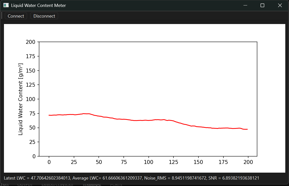
Interface Optimization<
Low Pass Filter<
# The new data is an exponential average of the oldest ones and the new computed signal
self.ydata[-1] = LOW_PASS*self.signal + (1-LOW_PASS)*self.ydata[-2]
Statistical informations computation<
# Compute statistical information over the data buffer
self.noise_rms = np.std(self.ydata)
self.mean_signal = np.mean(self.ydata)
self.SNR = self.mean_signal/self.noise_rms
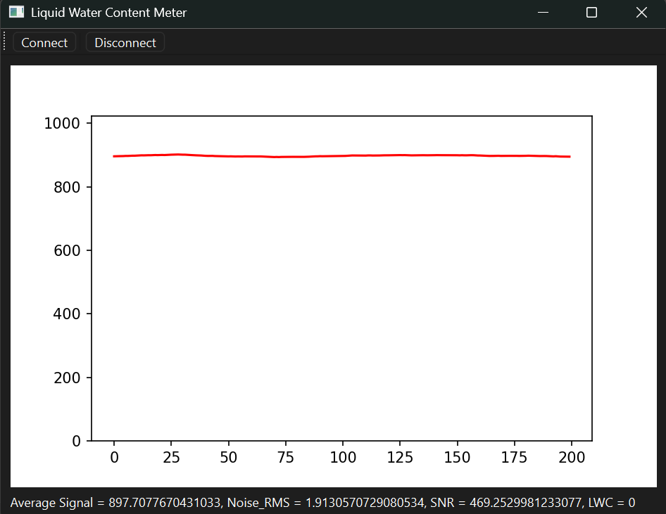
Layout and Statistics Display<
        # Create Widgets and Layout
        layout = QVBoxLayout()
        self.canvas = MplCanvas(self, width=5, height=4, dpi=100)
        self.mathlabel = QLabel("No Data")
        layout.addWidget(self.canvas)
        layout.addWidget(self.mathlabel)
        widget = QWidget()
        widget.setLayout(layout)
        self.setCentralWidget(widget)
def _refresh_plot(self):
    # Called by the UI thred timer. Draws only if necessary (i.e. dirty data).
    if not self._dirty:
        return
    self._dirty = False
    self._plot_ref.set_ydata(self.ydata)
    self.canvas.draw_idle()
    self.mathlabel.setText(f"Average Signal = {self.mean_signal}, Noise_RMS = {self.noise_rms}, SNR = {self.SNR}, LWC = {self.LWC}")
Toolbar, Connect and Disconnect Buttons<
# Create Toolbar
toolbar = QToolBar("Main Toolbar")
self.addToolBar(toolbar)

# Button
button_action = QAction("Connect", self)
button_action.setStatusTip("Connect serial port COM15")
button_action.triggered.connect(self._start_reader)
toolbar.addAction(button_action)

toolbar.addSeparator()

button_action2 = QAction("Disconnect", self)
button_action2.setStatusTip("Disconnect serial port COM15")
button_action2.triggered.connect(self.reader.stop)
toolbar.addAction(button_action2)
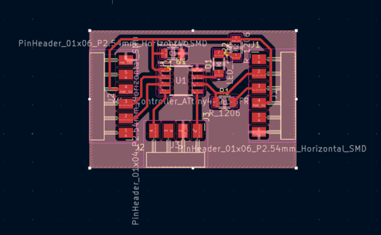
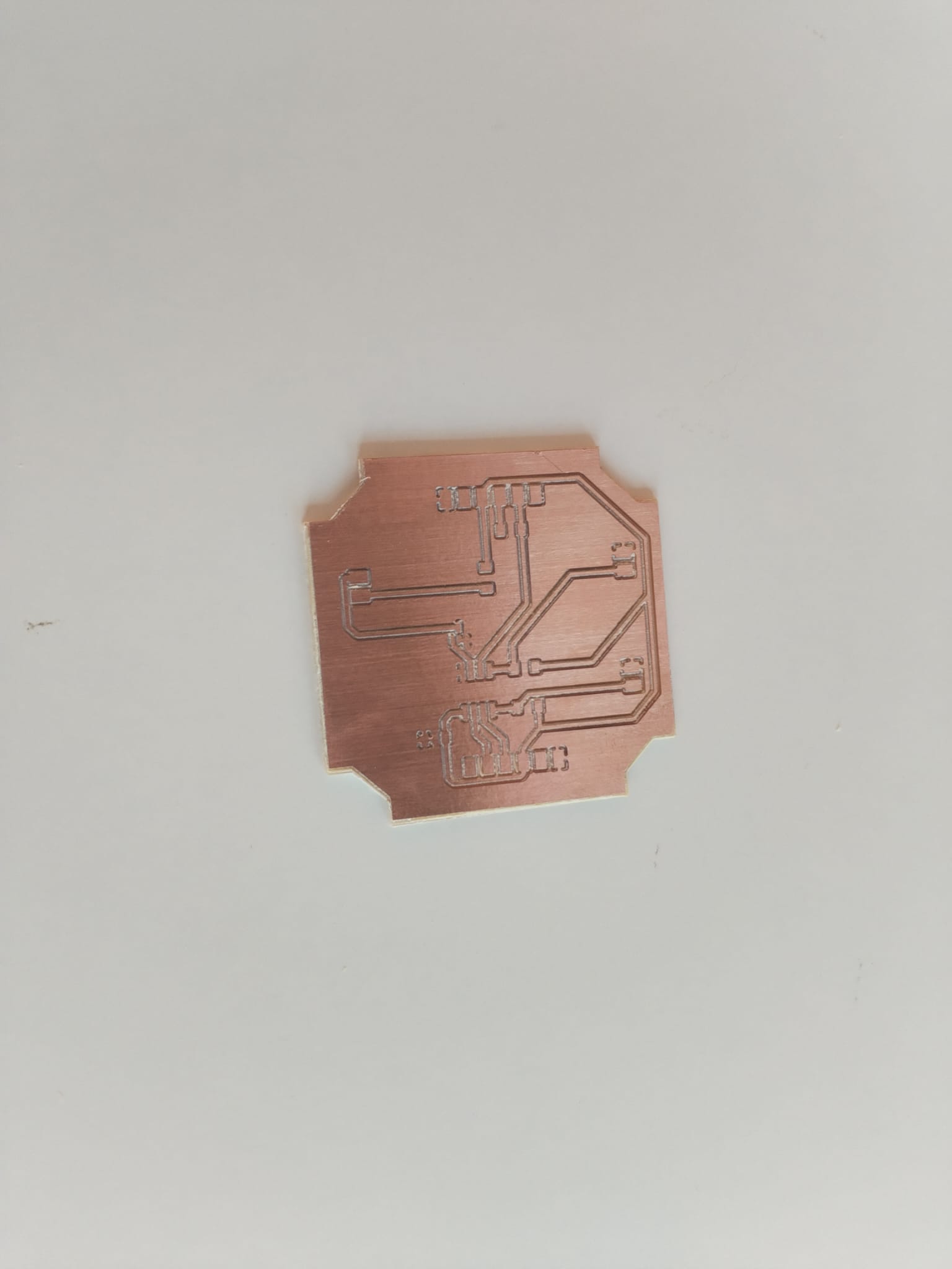
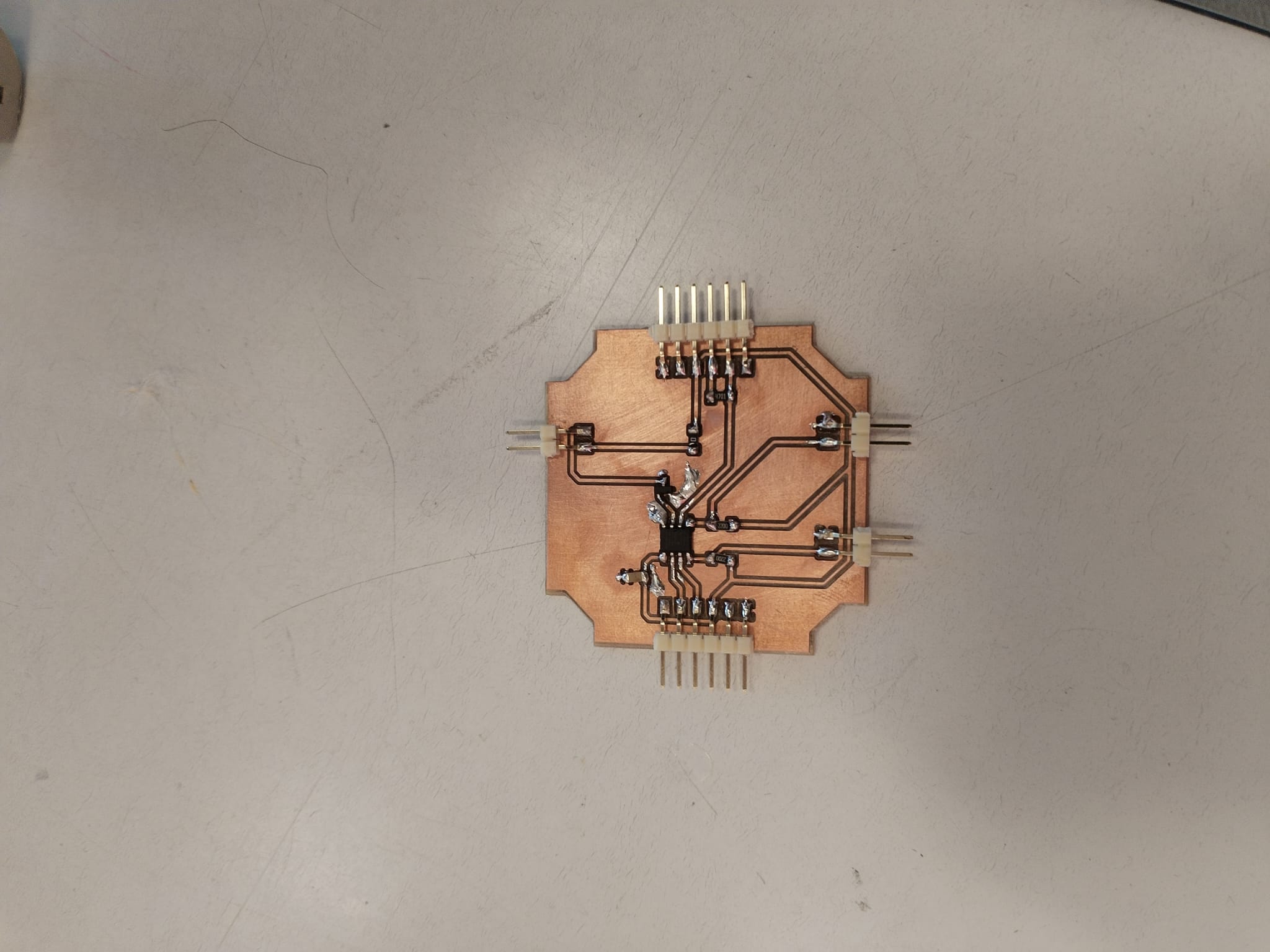
Hardware optimization<
The required hardware modifications are :
- Control the LED with a transistor
- Add a capacitor close the VCC as a filter
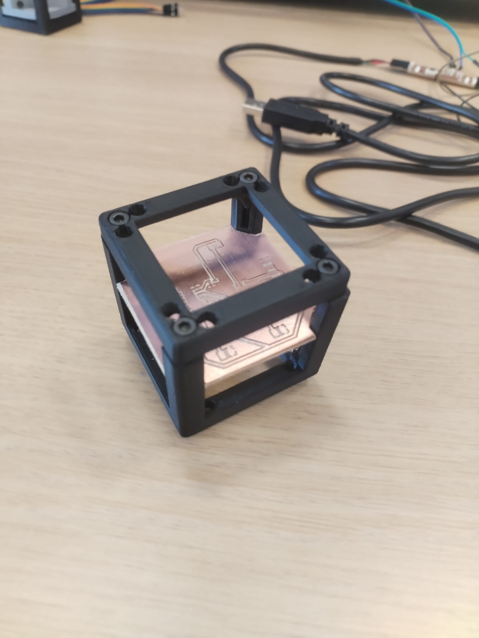
- Make the LED connector with a GND pin and a controllable pin
- Make the PCB easy to integrate in a UC2 container
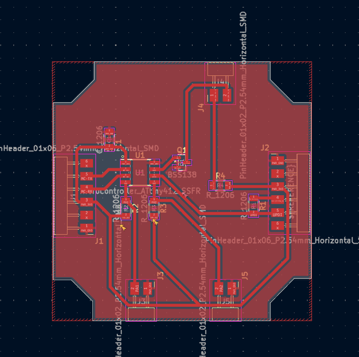
Note
This is the KiCAD Design.
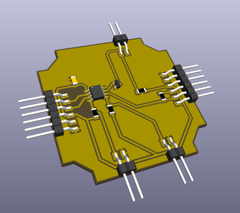
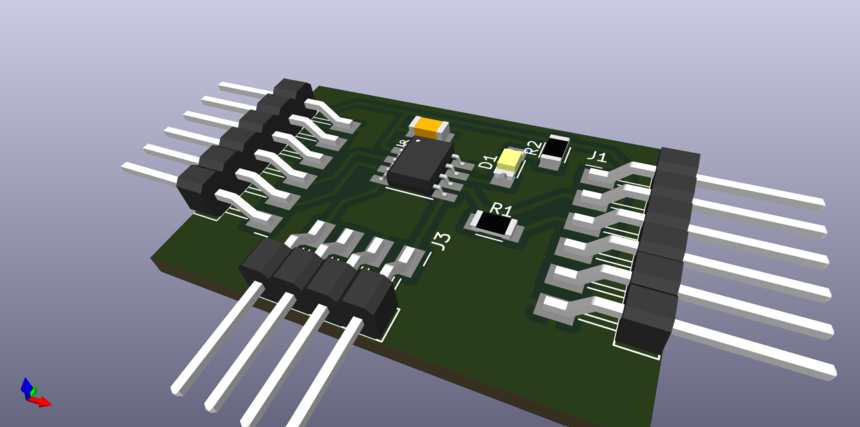
Note
This is the KiCAD 3D View.
Note
This is the KiCAD 3D View.
Note
This is the KiCAD 3D View.
Note
This is the KiCAD 3D View.
Note
This is the KiCAD 3D View.
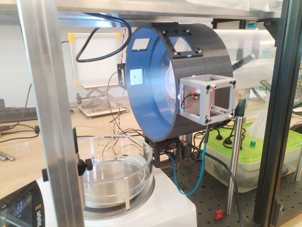
Week 18 : More System Integration<
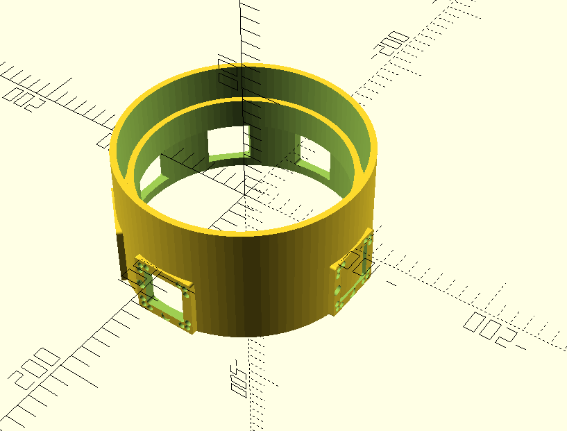
Few days left before final presentation ! I decided to give my project a "finished object" look. Therefore I designed a "crown" that would be inserted in the pipe and holding everything.
OpenScad Code
include<basepuzzleUC2.scad>;

module pipe(radius, thickness, height){
    difference () {
        cylinder(h = height, r = radius, center = true);
        cylinder(h = height, r = radius - thickness, center = true);
    }
}

module crown(r, th, h1, h2, a, e){
    union(){
        union(){
            translate([0,0,h1/2])
            pipe(r+th, th, h1);
            translate([0,0,h2/2])
            pipe(r-th-e/2, th, h2);
        }
        union(){
            translate([0,0,th/2])
            pipe(r + th,3*th,th);
            translate([0,0,-a/2])
            pipe(r + th,th,a);
        }
    }
}

module round_square_window(angle){
difference(){
rotate([0,0,angle])
        translate([0,-r,0])
            translate([0,0,-a/2])
                rotate([90,0,0])
                    cube([b,b,2*th],center=true);
    difference(){
        translate([-b/2,0,-b/2])
        rotate([0,0,angle])
        translate([0,-r,0])
            translate([0,0,-a/2])
                rotate([90,0,0])
                    cube([2*r1,2*r1,2*th],center=true);
        translate([-(b/2-r1),0,-(b/2-r1)])
        rotate([0,0,angle])
        translate([0,-r,0])
            translate([0,0,-a/2])
                rotate([90,0,0])
                    cylinder(h=2*th,r=r1,center=true);
    }
    difference(){
        translate([b/2,0,-b/2])
        rotate([0,0,angle])
        translate([0,-r,0])
            translate([0,0,-a/2])
                rotate([90,0,0])
                    cube([2*r1,2*r1,2*th],center=true);
        translate([(b/2-r1),0,-(b/2-r1)])
        rotate([0,0,angle])
        translate([0,-r,0])
            translate([0,0,-a/2])
                rotate([90,0,0])
                    cylinder(h=2*th,r=r1,center=true);
    }
    difference(){
        translate([b/2,0,b/2])
        rotate([0,0,angle])
        translate([0,-r,0])
            translate([0,0,-a/2])
                rotate([90,0,0])
                    cube([2*r1,2*r1,2*th],center=true);
        translate([(b/2-r1),0,(b/2-r1)])
        rotate([0,0,angle])
        translate([0,-r,0])
            translate([0,0,-a/2])
                rotate([90,0,0])
                    cylinder(h=2*th,r=r1,center=true);
    }
    difference(){
        translate([-b/2,0,b/2])
        rotate([0,0,angle])
        translate([0,-r,0])
            translate([0,0,-a/2])
                rotate([90,0,0])
                    cube([2*r1,2*r1,2*th],center=true);
        translate([-(b/2-r1),0,(b/2-r1)])
        rotate([0,0,angle])
        translate([0,-r,0])
            translate([0,0,-a/2])
                rotate([90,0,0])
                    cylinder(h=2*th,r=r1,center=true);
    }
}
}

$fn=100;

//Centimeters
e=1;
r=90+e/2;
h1=50;
h2=25;
th=5;
a=50;
b=34;
r1=2;

difference() {
    union(){
        rotate([0,0,180])
            translate([0,-r-th+1,0])
                translate([0,0,-a/2])
                    rotate([90,0,0])
                      baseplate_no_puzzle();

        rotate([0,0,135])
            translate([0,-r-th+1,0])
                translate([0,0,-a/2])
                rotate([90,0,0])
                    baseplate_no_puzzle();

        rotate([0,0,90])
            translate([0,-r-th+1,0])
                translate([0,0,-a/2])
                    rotate([90,0,0])
                        baseplate_no_puzzle();

        rotate([0,0,45])
            translate([0,-r-th+1,0])
                translate([0,0,-a/2])
                    rotate([90,0,0])
                        baseplate_no_puzzle();

        rotate([0,0,0])
            translate([0,-r-th+1,0])
                translate([0,0,-a/2])
                    rotate([90,0,0])
                        baseplate_no_puzzle();

        rotate([0,0,-90])
            translate([0,-r-th+1,0])
                translate([0,0,-a/2])
                    rotate([90,0,0])
                        baseplate_no_puzzle();

        crown(r, th, h1, h2, a, e);
    }
    union(){
        round_square_window(180);
        round_square_window(135);
        round_square_window(90);
        round_square_window(45);
        round_square_window(0);
    }
}
Week 18 : Calibration, Back to Interface<