Week2: Computer-aided Design
Introduction Computer Aided Design forms an important part in digital design and digital fabrication. My history with computer aided design began in …
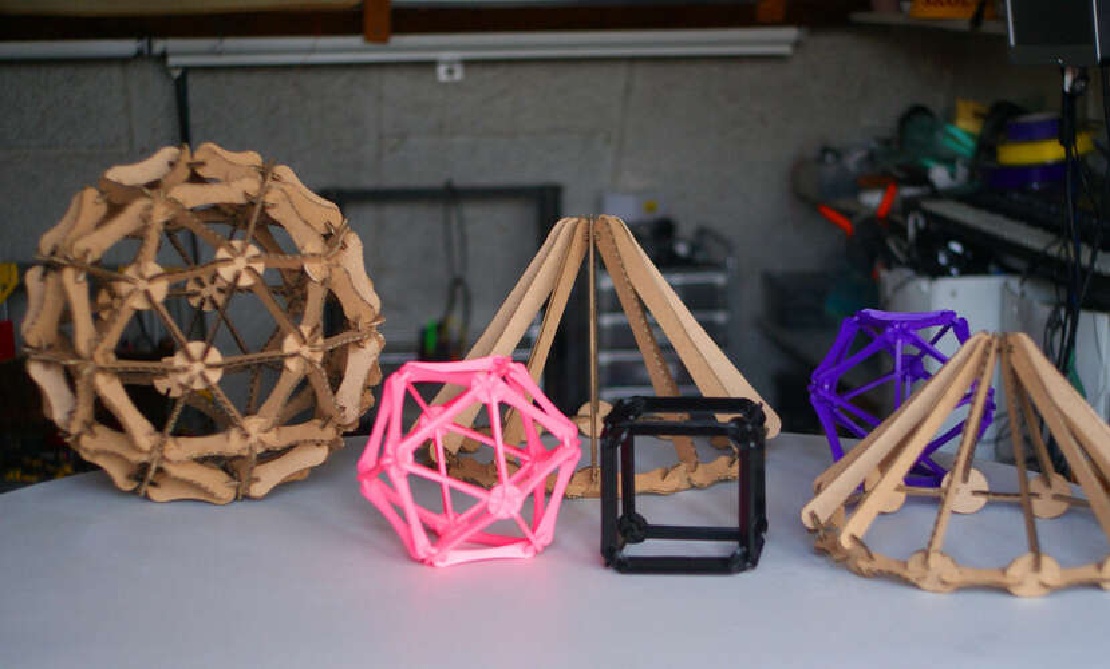
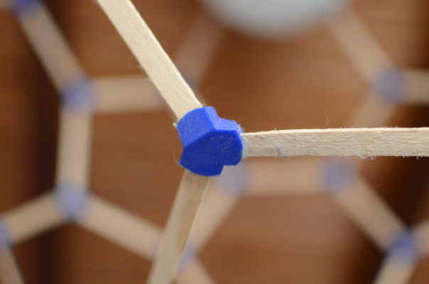
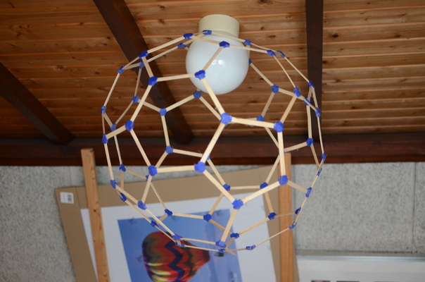
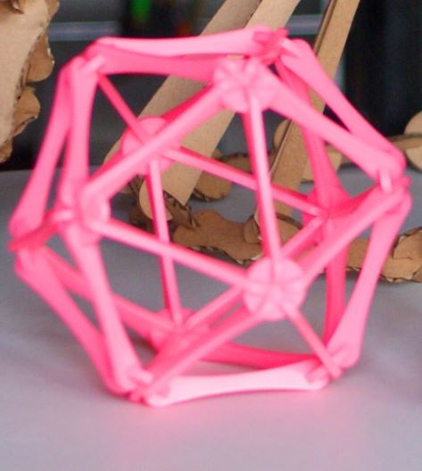
A couple of years ago I designed a construction kit where 3d printed “vertices”, held together with popsicle sticks, would build a 3d structure.
 |
 |
 |
|---|---|---|
| The vertex was made in openSCAD… | …and by combining 60 vertices… | … a sphere would emerge |
I was fascinated by the notion that by storing the three 3d vectors in a single shape, an entire geometric volume would emerge, just by following simple rules during assembly. I wanted to do more shapes but ultimately, calculating the angles for each geometric figure seemed like too much trouble. But I started wondering:
Can any mesh based geometric shape be made into a construction kit?
I never took the time to pursue this idea but I intended to put in the effort at FabAcademy. To fit the assignment for “Week 3: Computer Controlled Cutting”, I changed the initial question to:
Can any mesh based geometric shape be made into a 2D press fit kit?
A question that might rise is wether such a solution doesn’t already exist. Although there are many solutions where meshes are sliced into 2d planes to be reassembled, I have seen no technique that also takes into account the topology of the mesh. I would like to try to recreate the actual mesh in 3D because I like the aesthetic and it takes less material to reach a similar volume, compared to slicing techniques.
The end result for this assignment had to meet a couple of requirements:
To create this I had to learn: -creating python scripts for Blender -to apply 3d linear algebra, trigonometry and some graph theory to meshes -to generate pleasing geometric shapes in OpenSCAD -to control the laser-cutter -to find the best settings and properties for the laser-cutter
The result of this exercise is a combination of scripts that tie together the features of Blender and OpenSCAD to generate a 2D construction kit from practically any 3d mesh as it’s input.
 |
|---|
| A python script in Blender analyses the mesh and OpenSCAD uses the analysis to generate geometry |
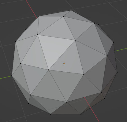
I tested the script on multiple shapes, of which a ico-sphere of tesselation-level 2 was the most complicated one to assemble
 |
 |
|---|---|
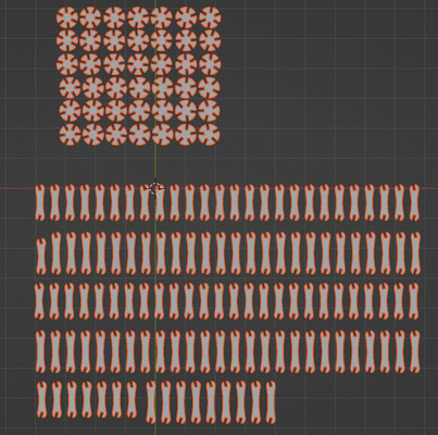
| An ico-sphere in blender | The geometry generated by the script |
 |
|---|
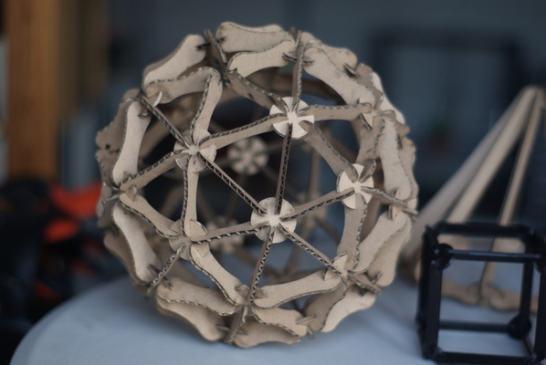
| The final result |
I was happy enough with the result I presented it voluntarily in the open review.
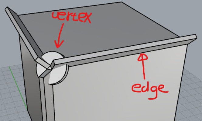
Having some experience programming and 3d geometry I know a 3d mesh has a data structure similar to a graph. Meshes consist of the following components:
| Term | Explanation | Image | data structure |
|---|---|---|---|
| vertex | 3d points in space that make up the shape | 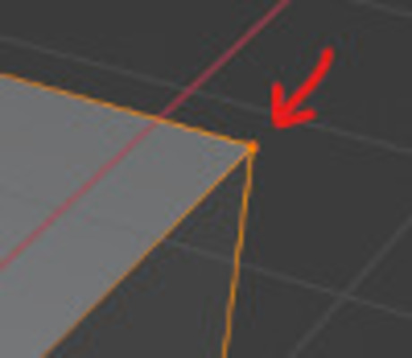 |
vertex = [x,y,z] |
| edge | indices of the vertices that are connected | 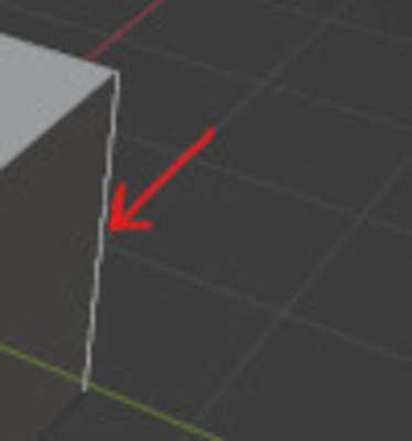 |
edge = [iVertex0, iVertex1] |
| face | indices of the vertices that, together, span a 3d region | 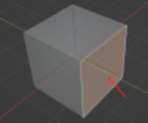 |
face = [iVertex0, iVertex1, iVertex2, ...] |
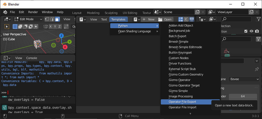
Blender has a powerful scripting engine. Most of its user-interface is written in python and is run by the scripting engine. To extend functionality, developers can write scripts right in the Blender interface. To get started, I opened a template script from within the scripting part of Blender.
 |
|---|
| I started with a template for an Export function |
This would give me a nice start to begin writing the export-to-openscad functionality. I changed the generic text-file export code to:
class ExportPFKData(Operator, ExportHelper):
    """Generate vertex and edge info to be used by OpenSCAD to generate 2d vertices and edges"""
    bl_idname = "export_test.some_data"
    bl_label = "Export PFK Data"

    filename_ext = ".scad"

    filter_glob: StringProperty(
        default="*.scad",
        options={'HIDDEN'},
        maxlen=255,
    )

    def execute(self, context):
        return export_connected_vertices(context, self.filepath)
The following code was needed to get to the internal data of the selected geometry in Blender:
# get selected mesh
mesh = bpy.context.selected_objects[0].to_mesh()
Important properties for this project were:
| Data | Representation |
|---|---|
mesh.vertices |
The entire array of vertices, each represented as a Vertex object |
mesh.vertices[0].co |
The coordinate of a single vertex represented as a Vector object |
mesh.vertices[0].index |
The index of the vertex, good to know when using foreach for the vertex array |
mesh.edges |
The entire array of edges, each represented as an Egde object |
mesh.edge[0].vertices |
An array of two integers, representing the indices of two vertices in the vertex array |
mesh.edge[0].index |
The index of the edge |
To know how to represent a “vertex”-part in my 2d kit, I needed to know what vertices were connected to each vertex in the mesh. For this I could use the edge data.
The algorithm looks like this in pseudo code
Create an array with empty lists, the size of the amount of vertices in the mesh

For each edge:
    find the list at the index found in the first element of the edge-vertex-index-array and
        append the edge index
        append the second element of the edge-vertex-index-array
    find the list at the index found in the second element of the edge-vertex-index-array and
        append the edge index
        append the first element of the edge-vertex-index-array
This way, all connected vertices are stored in the resulting list. The final python code would be like:
# creates a list of all connected vertices per vertex.
# the first index in each entry is the vertex index itself, subsequent indices are indices of
# connected vertices
def get_connected_vertices(mesh):

    # Find the amount of vertices
    nVertices = len(mesh.vertices)
    # Preallocate an list of lists, already filled with a vertex index
    connectedVertices = [[iVertex] for iVertex in range(nVertices)]

    # for all the edges
    for edge in mesh.edges:
        connectedVertices[edge.vertices[0]].append(edge.index)
        connectedVertices[edge.vertices[0]].append(edge.vertices[1])
        connectedVertices[edge.vertices[1]].append(edge.index)
        connectedVertices[edge.vertices[1]].append(edge.vertices[0])

    return connectedVertices
For a simple cube, the resulting list would look like:
# connectedVertices for a cube, each line representing:
#vertexIndex, edgeIndex, connected vertexIndex, edgeIndex, connected vertexIndex, edgeIndex, connected vertexIndex,
connectedVertices = [
    [0, 0, 2, 1, 1, 10, 4],
    [1, 1, 0, 2, 3, 11, 5],
    [2, 0, 0, 3, 3, 4, 6],
    [3, 2, 1, 3, 2, 5, 7],
    [4, 7, 6, 9, 5, 10, 0],
    [5, 8, 7, 9, 4, 11, 1],
    [6, 4, 2, 6, 7, 7, 4],
    [7, 5, 3, 6, 6, 8, 5]
]
Using this list, I could then find the directions of each connected vertex. The directions were stored as a normalized vector for each vertex:
#creates array containing:
# first 3 elements are the position for the pivot vertex
# first 3 elements are the direction for the pivot vertex
# subsequent elements are x, y and z for each connected vertex w.r.t. pivot vertex
def create_vertex_array(mesh, vertexIndices):

    firstVertex = mesh.vertices[vertexIndices[0]]
    vertexArray = [firstVertex.co, firstVertex.normal] #store position and normal

    averageOutDir = mathutils.Vector((0.0, 0.0, 0.0))

    # for each subsequent vertex index
    for iVertexIndex in range(1, len(vertexIndices),2):
        iEdge = vertexIndices[iVertexIndex]
        iVertex = vertexIndices[iVertexIndex+1] #find the vertex location for this vertex
        vertexCo = mesh.vertices[iVertex].co #set first vector to be vertex position
        #calculate the normalized outgoing direction w.r.t. the pivot vertex
        outDir = (vertexCo - firstVertex.co).normalized()
        vertexArray.append(iEdge)
        vertexArray.append(outDir) # add the direction vector components to the list
        averageOutDir += outDir

    # calculate the average direction of all outgoing vertices
    averageOutDir /= len(vertexIndices)-1
    averageOutDir.normalize()
    # replace vertex normal with average output direction
    # Choose best strategy, comment line if other strategy works better
    vertexArray[1] = averageOutDir

    return vertexArray
For each “vertex”-part un my construction kit to have an optimal angle, I decided to calculate the “direction” of the vertex. Vertices are points in 3d space and have no direction, but a direction can be derived from the connected geometry. Often an average of the connected face normals is used for lighting purposes but I decided to calculate the direction of the vertex to be the normalized average of all directions toward the connected vertices. This would minimize the chance of having edged that would coincide with the direction of the vertex, therefore make it impossible to find a working angle for that edge.
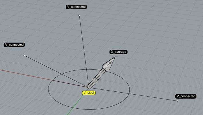 |
|---|
The average of connected vertex directions, d_avg, is used to calculate pivot-vertex “direction” |
The average direction d_avg is calculated by taking the sum of all direction vectors v_i pointing towards the connected vertices from the pivot vertex v_p and dividing the result by the amount of connected vertices to that pivot-vertex:
\[d_{avg}=\frac{1}{n}\sum_{i=1}^{n}\overrightarrow{{V}_{i}} - \overrightarrow{V}_{pivot}\]
For a cube, one vertex would yield the following data:
vertexArray = [
    Vector((-1.0, -1.0, -1.0)), # the vertex to analyze
    Vector((0.5773503184318542, 0.5773503184318542, 0.5773503184318542)), the direction of the vertex
    0, Vector((0.0, 1.0, 0.0)), # connected vertex index and normalized direction
    1, Vector((0.0, 0.0, 1.0)), # connected vertex index and normalized direction
    10, Vector((1.0, 0.0, 0.0)) # connected vertex index and normalized direction
]
Having the data like this for each vertex and having data for all edges (vertex indices and length) would be enough to reconstruct the mesh in 2D in OpenSCAD. I converted all the data I needed to openSCAD variables so they could be imported in my main openSCAD program as external data. A final data-file for a cube would look like this:
vertexData = [
# pivot vertex position, pivot vertex direction, edge index, vertex direction, edge index, vertex direction, edge index, vertex direction,
[[-1.0, -1.0, -1.0], [0.577, 0.577, 0.577], 0, [0.0, 1.0, 0.0], 1, [0.0, 0.0, 1.0], 10, [1.0, 0.0, 0.0]],
[[-1.0, -1.0, 1.0], [0.577, 0.577, -0.577], 1, [0.0, 0.0, -1.0], 2, [0.0, 1.0, 0.0], 11, [1.0, 0.0, 0.0]],
[[-1.0, 1.0, -1.0], [0.577, -0.577, 0.577], 0, [0.0, -1.0, 0.0], 3, [0.0, 0.0, 1.0], 4, [1.0, 0.0, 0.0]],
[[-1.0, 1.0, 1.0], [0.577, -0.577, -0.577], 2, [0.0, -1.0, 0.0], 3, [0.0, 0.0, -1.0], 5, [1.0, 0.0, 0.0]],
[[1.0, -1.0, -1.0], [-0.577, 0.577, 0.577], 7, [0.0, 1.0, 0.0], 9, [0.0, 0.0, 1.0], 10, [-1.0, 0.0, 0.0]],
[[1.0, -1.0, 1.0], [-0.577, 0.577, -0.577], 8, [0.0, 1.0, 0.0], 9, [0.0, 0.0, -1.0], 11, [-1.0, 0.0, 0.0]],
[[1.0, 1.0, -1.0], [-0.577, -0.577, 0.577], 4, [-1.0, 0.0, 0.0], 6, [0.0, 0.0, 1.0], 7, [0.0, -1.0, 0.0]],
[[1.0, 1.0, 1.0], [-0.577, -0.577, -0.577], 5, [-1.0, 0.0, 0.0], 6, [0.0, 0.0, -1.0], 8, [0.0, -1.0, 0.0]]
];

 # first vertex index, second vertex index, edge length
 edgeData = [[2, 0, 2.0],[0, 1, 2.0],[1, 3, 2.0],[3, 2, 2.0],
    [6, 2, 2.0],[3, 7, 2.0],[7, 6, 2.0],[4, 6, 2.0],
    [7, 5, 2.0],[5, 4, 2.0],[0, 4, 2.0],[5, 1, 2.0]
    ];
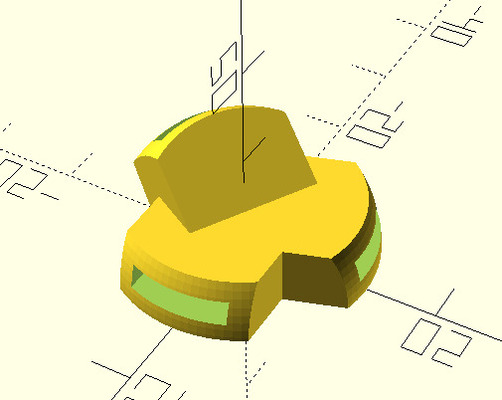
I decided the basic vertex shape should be a circle. This would give the vertex enough body to accommodate the slots for several edges. The amount of edges a single vertex could have depends on the size of the vertex and the thickness of the material.
 |
|---|
| A single corner of a cube was visualized in Rhino |
Once the data generated by blender was loaded into openSCAD, the vertex “direction” was used to transform each vertex and its connected vertices so it would lay “flat” on the xy-plane. This was done using the following process:
|
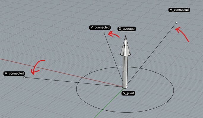 |
|---|---|
| Connected vertices with their average direction. | All connected vertices are transformed so the average direction points up (+z) |
In mathematical notation it might be something like:
\[ \overrightarrow{y} = \begin{pmatrix} 0.2 \\ -0.4 \\ 0.7 \end{pmatrix} \]
\[\overrightarrow{z}=\overrightarrow{d}_{avg}\]
\[\overrightarrow{x}=\overrightarrow{z} \times \overrightarrow{x}\]
\[T=\begin{bmatrix}\overrightarrow{x} & \overrightarrow{y} & \overrightarrow{z} \\\end{bmatrix}\]
\[{v}_{connected}^{'}={v}_{connected} * T^{-1}\]
Where d_avg is the average direction of all vertices. The y vector is chosen in a way to minimize the chance that this vector would coincide with the average direction vector.
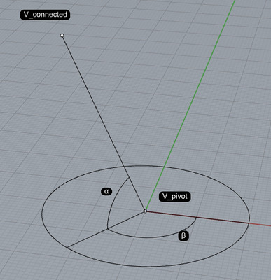 |
|---|
| To make the final shape of the vertex I had to calculate the angle the transformed connected vertex direction would make with the z-axis |
The z-axis angle beta was calculated using:
\[\DeclareMathOperator{\atantwo}{atan2} \beta=\atantwo(v_{y}, v_{x}) \]
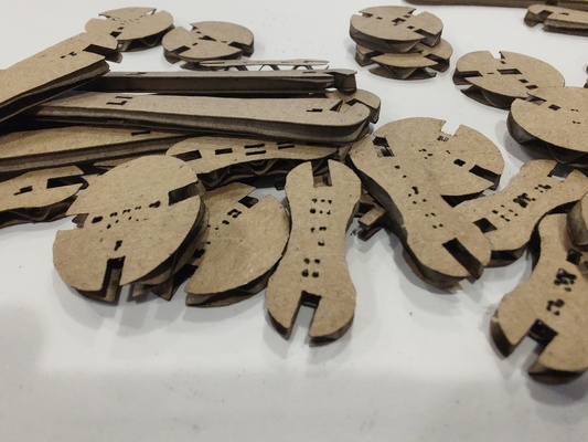
The edge would be an elongated shape, like a rectangle with circular ends. The length of the edge was collected from the information generated by Blender.
To have a more interesting shape I assembled an elongated shape using three circles.
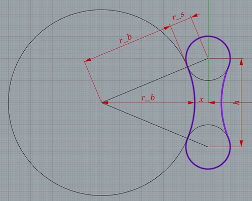 |
|---|
Two large circles at both sides, with radius r_b(ig) are placed between two smaller circles with radius r_s(mall). The distance x can be set by the user to be between 0 and r_s/2. h is the distance between the smaller circles |
From the given parameters r_s, x and h, r_b can be calculated:
\[r_b=\frac{h^2-4r_s^2 + 4x^2}{8r_s} \]
(Thanks Saco Heijboer, for helping me with this)
The angle of the slot would be calculated with the information from the transformed connected vertex direction data as angle alpha. This angle can be calculated by:
\[d_{xy}= \begin{pmatrix} d_x \\ d_y \\ 0 \end{pmatrix}\]
\[\alpha = \arccos {\frac{d \bullet d_{xy}}{\left|d\right|\left|d_{xy}\right|}} \]
The angle alpha is then used to subtract a slot shape from the edge.
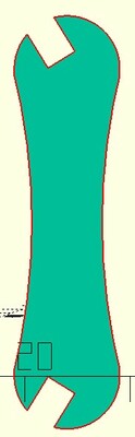 |
|---|
| This is done at both ends to get a wrench shape |
The first mesh shape I tested was a simple cube, because it would be possible for me to read and interpret the resulting data from the Blender export script. At this point I was not able to test it with the laser-cutter so I had to generate the parts using a 3d printer.
 |
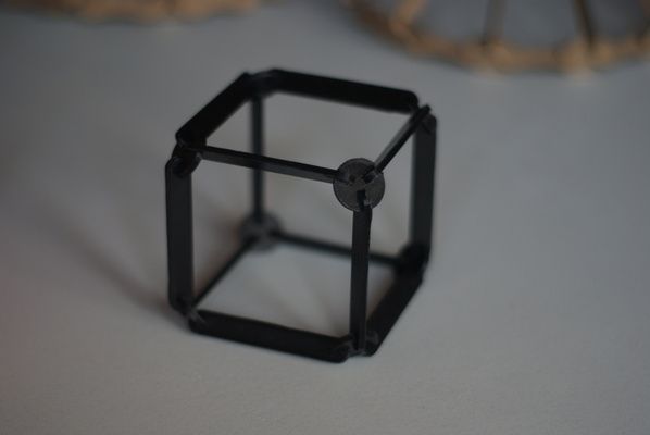 |
|---|---|
| The output of the OpenSCAD script | The resulting shape |
Pleased with the result I ran the script on an icoSphere at a tesselation level of 1:
 |
 |
|---|---|
| The output of the OpenSCAD script | The resulting shape |
Quite pleased with the 3d printed results I went to create other shapes with the laser-cutter.
The LaserCutter at the Waag is a BRM1612 and has the following characteristics:
The control board was replaced and it is now operated by LightBurn software. LightBurn will accept SVG files without too much inconvenience.
Laser-cutters operate by accurately moving an assembly consisting of lenses and mirrors to reflect a beam, originating from the laser tube and focus it onto the material. To successfully cut any material, one has to take into account a couple of parameters:
| Parameter | Explanation |
|---|---|
| Type of material | Acrylic, cardboard, plywood, etc. If it doesn’t give a colorful flame and dangerous fumes, it can be cut |
| Material thickness | Measured in mm |
| Speed | Measured in mm/min, the speed of the moving assembly |
| Power | The amount of power output by the laser, measured in % from its maximum. Laser tubes degrade with use |
| Focus | A laser beam might seem parallel but actually has a focal-point at which the beam can most optimally cut through material |
Also, linear and nonlinear deformations of the sheet material mus be taken into account.
Most of the decisions are all about speed and power. Higher speeds will make the process faster, but will also result in less laser energy transferred to your cut. High power will give a higher chance of charring the material while lower power will make it harder for the machine to cut material. As a rule of thumb, use the highest speed with the lowest power necessary to cut material.
To laser cut anything, the following procedure has to be followed:
| Step | Image |
|---|---|
| Turn on the machine by turning the key | 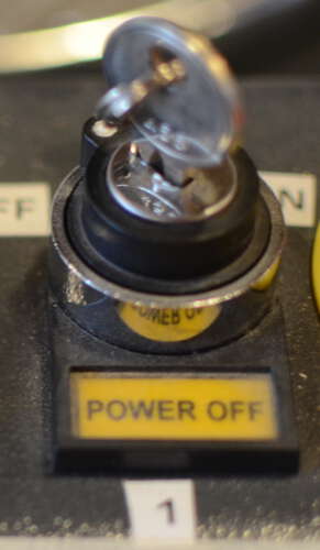 |
| Turn on the machine by pressing the button | 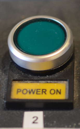 |
| The laser assembly will home and then move to the last position | |
| Log in and start the LightBurn software | |
| Insert a USB drive | 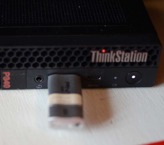 |
| Load an SVG into LightBurn | |
| Decide what parts of the work will be cut or engraved differently by putting parts in layers | |
| Set the speed and the power for each layer, according to the material and the desired effect (cutting or engraving) | |
| Decide the origin of the piece. This will be the starting point of the laser | |
| Insert the material | |
| Make sure the material is as flat as possible. Use bricks if necessary | 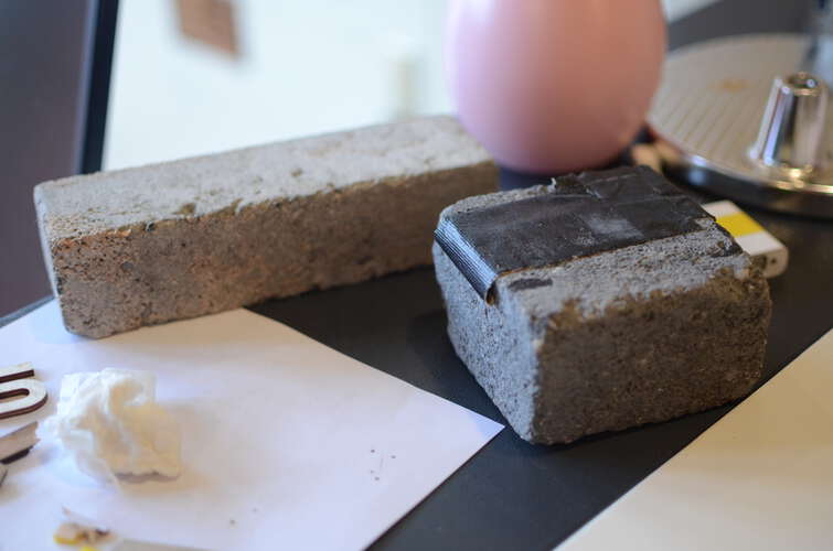 |
| Use the focus-block to adjust the height of the laser assembly and ensure optimal focus | 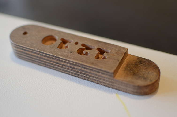 |
Perform a bounding-box test (frame) to be sure the piece fits the material and the assembly doesn’t hit bricks |
|
| Close the lid | |
| Turn on the fume extractor | 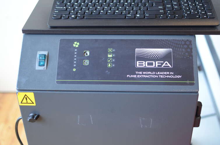 |
| Turn on the laser by turning knob no.3 | 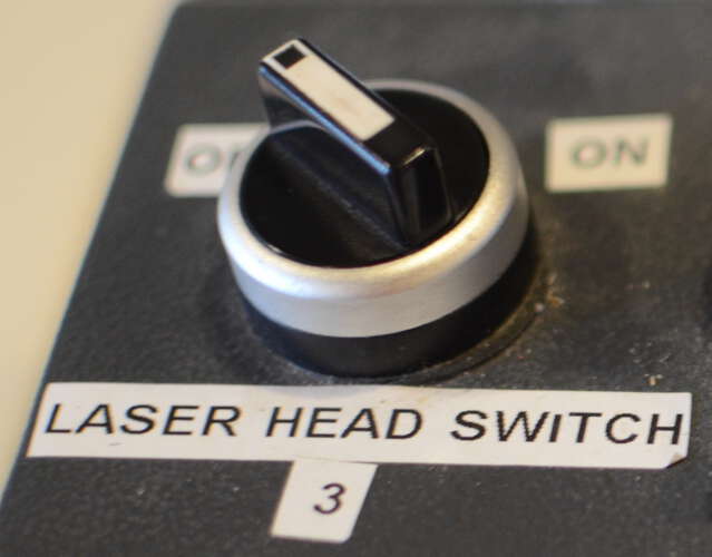 |
| Start the machine in LightBurn | |
| Never leave the red area | |
| When it’s finished, leave the lid on for a minute to extract the fumes | |
| Open the lid, remove your work and clean unused parts. Small parts can be vacuumed |
As thin as it might seem, a laser has some width and burns away material on both sides of the cut. There is actually some material lost and to make a well fitting press-fit, one has to know how much material is actually burned away in order tom compensate for that.
To determine the kerf, one can cut a piece of material with a known intended width and measure the resulting width from the actual cut piece. The measurement becomes more accurate if multiple pieces are cut and the total loss of material is divided by the amount of pieces that were cut.
The material we set out to test was a piece of plywood, measured to be 3.2mm thick.
 |
|---|
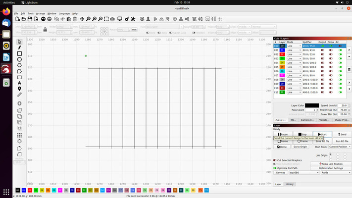
| A testpiece was made by drawing the lines directly in LightBurn |
 |
 |
|---|---|
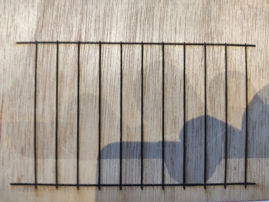
| At power 40, speed 40, the laser did not cut through the material | At speed 30, power 60, the material was cut. |
Measuring all the pieces would yield a total width of 99.2. 11 cuts were made to cut out the pieces, but two cuts count for half the kerf because those were on their outside. For 10 cuts, 0.8 mm of the material was lost, so that will be 0.8/10 = 0.08mm per cut. SO for plywood the kerf is 0.08mm.
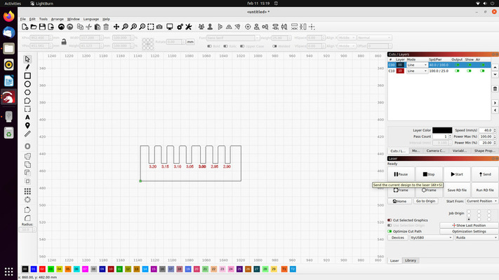
To test the press-fit for the plywood material we drew a small test-jig in Rhino, which we could cut twice. We decided to engrave the width of the slots so we could easily read which width would give the best fit. A chamfer of 0.5mm was added to the slots in order to help the slots to slide into place.
 |
 |
|---|---|
| The test-jig loaded into LightBurn | Two jigs fitted best at 3.2mm |
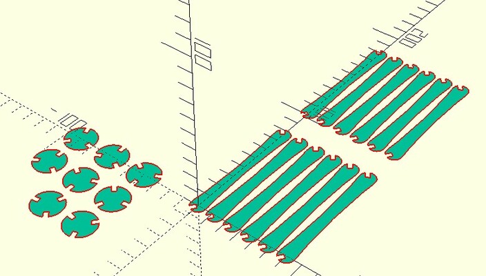
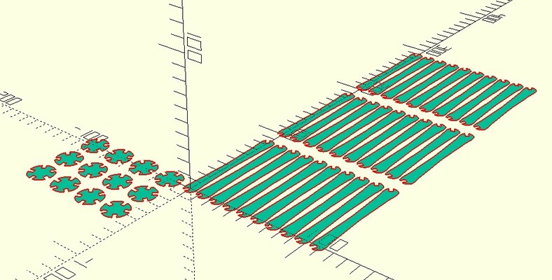
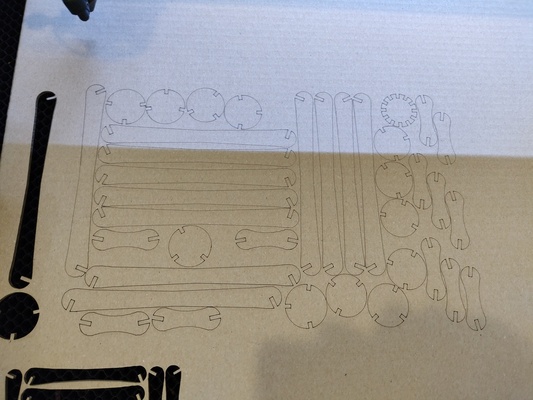
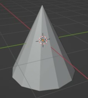
Once the press-fit was tested and the kerf was known I could commence using the lasercutter for my mesh-press-fit-kit project. I started out by generating a cone. This was the first shape I tried with different lengths, angles and vertices. Up until now all shapes were uniform, needing only one type of edge and one type of vertex.
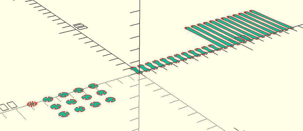 |
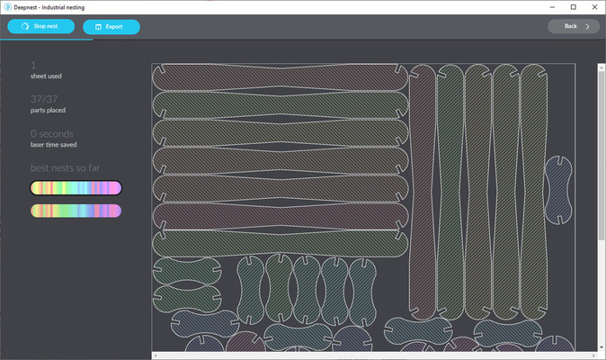 |
|---|---|
| Cone kit in openscad | Deepnest for optimization |
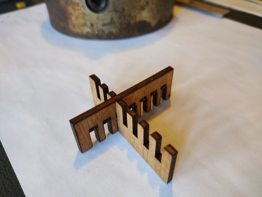
The material used for the cone was cardboard.
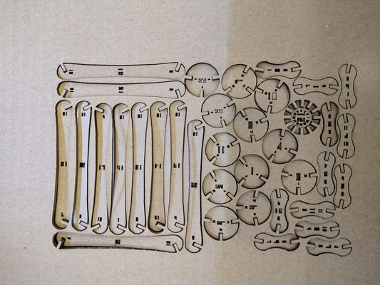 |
 |
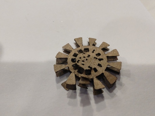 |
|---|---|---|
| Kit right out of the lasercutter | Loose parts | Way too small for cardboard |
It turned out I was way too optimistic regarding the size of the kit. I thought to save material by starting out small, but the internal structure of the material wold prevent it from forming a strong fit. The second try was roughly a factor 3 larger.
 |
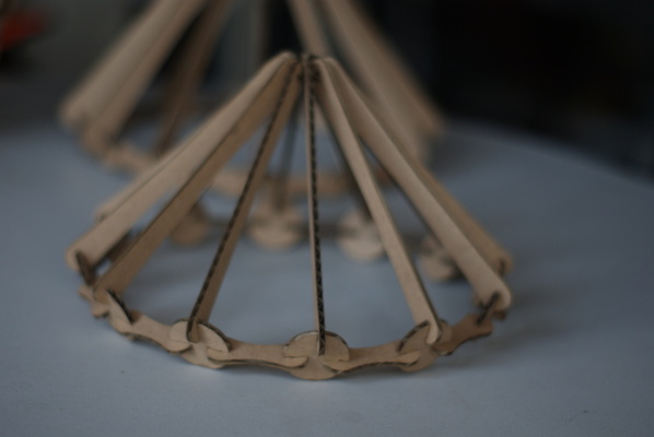 |
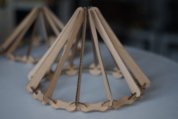
|---|---|
| The kit in the lasercutter | The resulting cone |
The second try seemed to work quite fine. The slots were a bit too wide but the structure held together pretty well. A problem became apparent because this was the first shape to be non-uniform. I assumed the vertices and the edges were perfectly in the center of all the laser cut shapes that make up the edges, but reality was different fro the perfect world of geometry. This resulted in the base of the cone being way to large. Eventually I made a small bugfix to the code in which the length of the edge gets compensated by the angle it makes with the vertex.
 |
 |
|---|---|
| The second cone was a bit better but still not resembling the original Blender cone. More work is needed. |
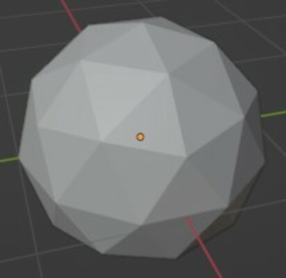
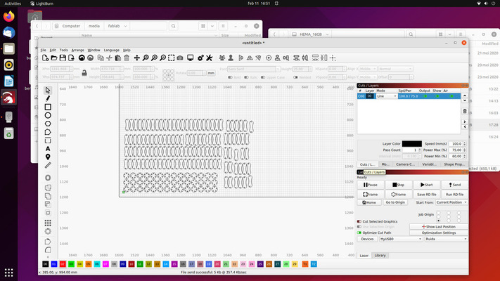
The second project on the laser-cutter was to make a larger, more complicated object on the lasercutter. Being only able to use a 3d printer before made me limited in the complexity of the shapes I could make, because it would take a very long time to make. On the lasercutter, a complex shape would take minutes instead of hours. I decided to do a larger ico-sphere so I wouldn’t run into trouble having different edge lengths and vertices.
 |
 |
|---|---|
| The icosphere in blender | The kit parts in LightBurn |
Assembling the sphere was quite a chore. There were two different kinds of edges, one slightly shorter than the other, and two different kinds of vertices, with 5 and with 6 slots. These had to be assembled in a specific manner in order to recrate the sphere.
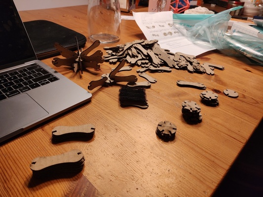 |
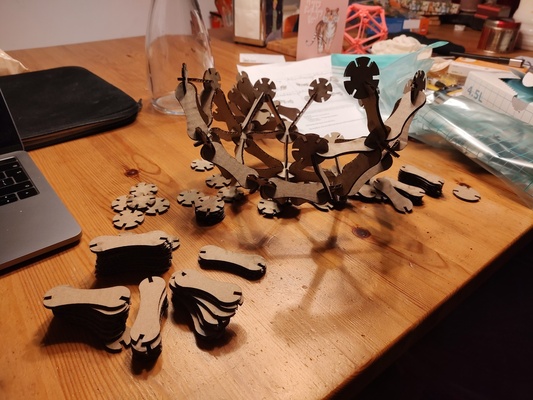 |
|
|---|---|---|
| The sphere parts | Assembling the sphere | The final result |
In order to generate more complex meshes, two improvements need to be made:
I wanted to try and generate an image to then cut with the vinyl cutter.I came up wit a little Processing sketch, generating a random maze from circles and rectangles.
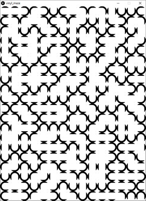 |
 |
|---|---|
| The output of the processing sketch | The resulting SVG from processing was unusable for cutting |
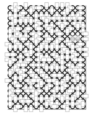
Using basic shapes resulted in am SVG file containing all those basic shapes. Every line would be a cutting path, making weeding an absolute chore. I tried to generate an SVG from the resulting bitmap from Processing but wasn’t happy with the result. I also sacrificed a little time to find a Processing library that allowed me to perform boolean operations on simple shapes. When that proved to be difficult I realized that OpenSCAD would fit my needs perfectly, so I ported the algorithm to OpenSCAD.
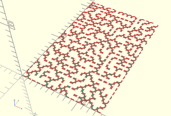 |
|---|
| The final maze in openSCAD |
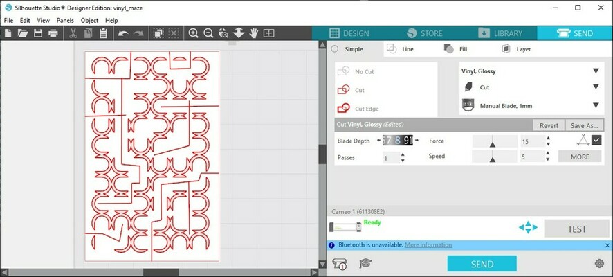
I did’t have time to perform the cutting at de Waag so I decided to use my own Vinyl cutter, a first generation Silhouette Cameo.
Silhouette Studio is the software that I used to control the cutting machine. It allowed me to import the SVG file exported from OpenSCAD. Based on the material I wanted to cut I can manually set the cutting depth by removing the knife from the device and turning a screw to a set position. I set mine to 8.
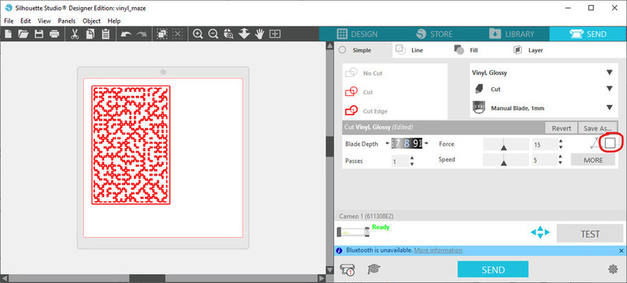 |
|---|
| I enabled the option to over-cut sharp corners, to make sure weeding was possible |
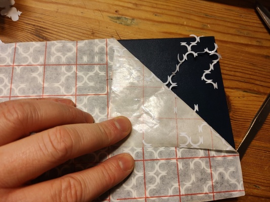
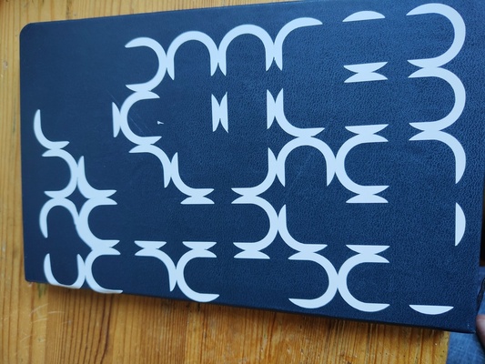
The final result was a sticker, from which I had to remove all the material I didn’t want to be part of my final design. This process is called “weeding”
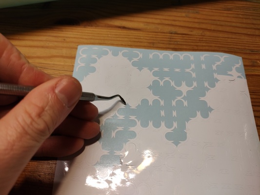 |
 |
|---|---|
| Weeding | The weeded result |
The weeding process wasn’t pleasurable at all because I chose to have the walls of the maze to be quite thin. A lot of material needed to be removed, ripping away pieces that I actually wanted to stay. Eventually I manage to weed all the unwanted parts from the sticker and end up with almost all of the parts that I wanted to keep.
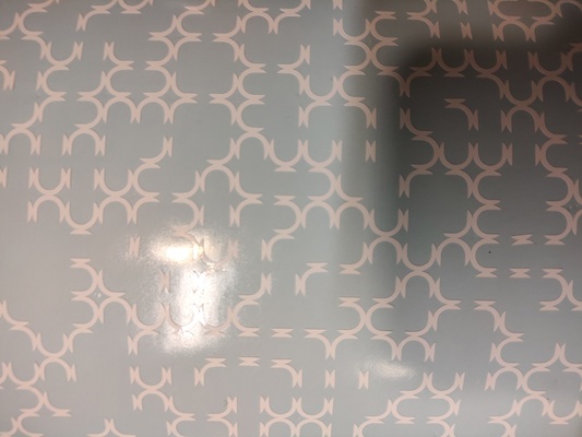
Next was the process of transferring the design to my notebook.
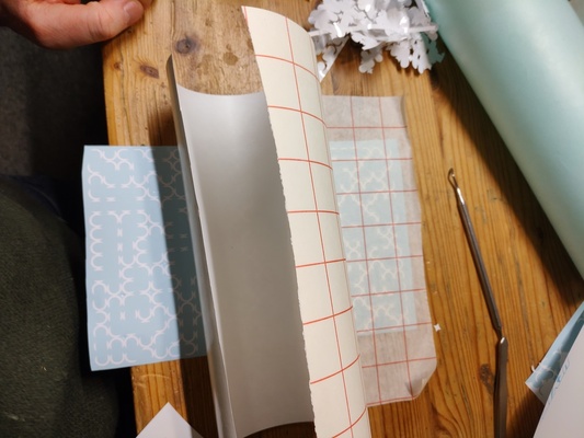 |
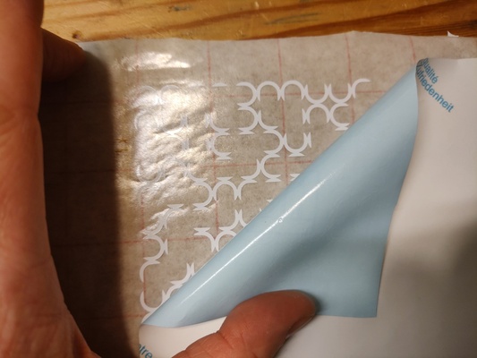 |
|---|---|
| I applied transfer-foil to the vinyl… | …and removed the backing. |
The result was quite painful. Sticking the design to my notebook I realized I probably had to degrease the surface with alcohol first. Furthermore, the really small loose parts were not inclined to stick to the surface at all.
 |
|---|
| The final result failed spectacularly |
The nest day I tried again. This time I kept the plotter settings the same but I made the design less intricate. Furthermore, I added extra cuts in the negative spaces in order to have smaller pieces to peel off.
 |
 |
|---|---|
| The extra cuts were added in Silhouette Studio | The result was transferred to the (degreased) surface, but it was very badly aligned |
The day after, I tried to do it one more time. This time I would take everything into account:
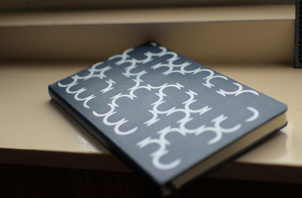 |
|---|
| I was finally happy with the result |
The end result for this assignment had to meet a couple of requirements:
It’s possible to make all platonic solids with just a couple of actions required. Tweaking the parameters for an optimal cut takes a bit longer.
Generated kits are entirely 2d.
Export from blender is one button-press. Importing in OpenSCAD takes no time at all. Assembling a laser-cut kit is quite a puzzle.
To create this I had to learn:
The Blender export script is written in Python. As an extra challenge for myself I tried to use as few for-loops as possible and use the built in string manipulation functionality as effective as possible.
Nothing too fancy but I am happy I could finally apply all that math they taught me in college.
I like the bone-like aesthetic of the edge-shapes.
I learned how to operate the lasercutter at the Waag fablab. It’ll take more time to actually be able to really get the grasp ot it’s settings.
I must admit that I started working on this assignment a bit earlier. It took quite some time and a lot of tweaking to get the system working. I wish I could have spent more time with the lasercutter in the lab.
One thing I definitely must do better next time is to make more pictures of the process. I was too enthralled with the work I completely forgot to log my progress, also because time at the lasercutter was limited.
In future assignments I have to find a way to make most of my time in the lab. I feel there’s hardly any room to make a mistake or to iterate. When somethings doesn’t work out, bad luck, your’re out of time. I’ll probably keep using my own equipment to make prototypes and make the final work in the lab. That’s how I can make mistakes in my own time and use the lab time efficiently.
Introduction Computer Aided Design forms an important part in digital design and digital fabrication. My history with computer aided design began in …
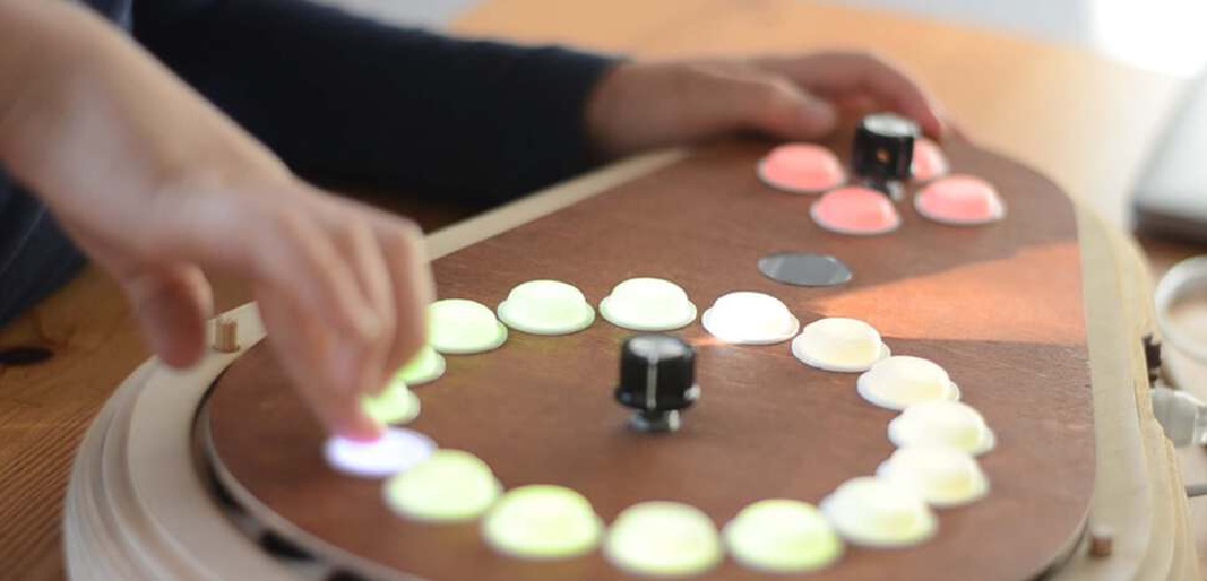
Final project Initial conception (Febuary 2022) Learning to play any musical instrument takes a very long time and a lot of effort. To enjoy music …