2. Computer Aided design

This week I designed the final project in 2D and 3D CAD. For 2D, we used Procreate and InkScape, and for 3D, I used Fusion360 and OpenSCAD.
Weekly Assignment Requirement
- model (raster, vector, 2D, 3D, render, animate, simulate, …) a possible final project,
- compress your images and videos, and post a description with your design files on your class page
Have you answered these questions?
- Modelled experimental objects/part of a possible project in 2D and 3D software
- Shown how you did it with words/images/screenshots
- Included your original design files
What I’ve done this week
-
Compress images and videos
-
Create a logo for the trash box that will be created for the final project.
-
Model the trash box to be created for the final project.
Compress images and videos
I will do my best not to go over 10MB and not enter the top 10.👍
Compress images I did this in Week01, but I’ll share it again
% brew install imagemagick
The following command compresses all the images in the directory under -path to 300x300 in a batch and uses the “-quality” option to determine the quality using a number between 1 and 100.
mogrify -path ./thm -resize 300x300 -quality 50 *.jpg
In Fabacademy, we need to process a large number of photos, so I would like to use the following commands to complete the processing in one shot.👍
If you want to process a single file directly, use the convert command.
convert -resize 300x300 -quality 100 ./sample1.jpg ./thm/sample1-300x300.jpg
Compress video
For macOS, you can also install this through homebrew.
% brew install ffmpeg
The following command will output input.mp4 as output.mp4 with quality 30.
ffmpeg -i input.mp4 -crf 30 output.mp4
-crf Select the quality for constant quality mode (from 0 to 63) (default 0)
Create an icon for the trash to be used in the final project
Create a trash icon with Procreate and convert it to vector format with Inkscape

First, Create an illustration of the logo using procreate. procreate
Procreate is my favorite drawing software!
This time, I used Inking studio pen to create the logo.

The logo to be created here will be cut using the cutting machine at week3 computer controlled cutting and will be attached to each trash box in the final project.
First, I will create four icons: battery, plastic, charcoalable trash, and non-charcoalable trash.
![]()
After painting the outline, you can drag and drop colors to paint the entire outline at once.

![]()
Done🔥
Convert the created icon data to vector data with Inkscape
Inkscape is a software for creating and editing vector images in a professional quality.
This tool is free to use and has features comparable to Adobe Illustrator.
In Week03, the cutting machine uses A4 size sheets, so this time I chose A4 size.

From the mac menu bar, click on path, and then click on Trace Bitmap.

I set it up as shown in the picture below.
Check Stack and remove background.Stack is for “Stack scans,Speckles is for “Suppress speckles,” Optimize is for “Optimize paths.

If you have only black line drawings like in the image, you can use “Simple scan” to trace the bitmap.

I did the same thing with four icons, as follows.

Done🔥
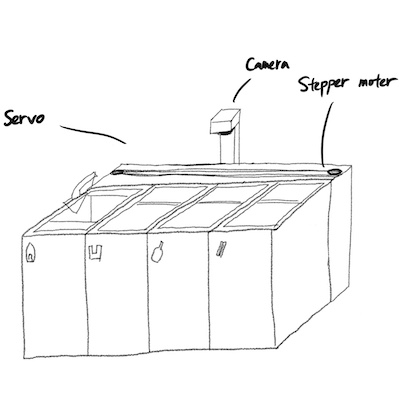
Model the trash box to be created for the final project.
To use Fusion360, first you need to create an Autodesk account.
The following link will take you to the Fusion360 download page. fusion360
First, let’s take a look at the basic tools.

Fusion360 basically does modeling by sketching on a plane in 2D and then extruding the sketch.
I did 3D modeling this final project drawing that I created in week01.

First, I created the parts for the trash box.
Select an XY plane and sketch in that plane.

Select Create => Rectangle => Center Rectangle

Specify size of Rectangle

Done👍

By entering the E key in this state, you can extrude a sketch.


Done👍
The next step is to draw a sketch on the top of the rectangle.
To do so, click on the top of the rectangle and select “Create a sketch”.


Make a sketch on the top of the rectangle.


By entering the E key in this state, you can cut a sketch.


Done🔥
Next, Line up the four trash box.
First of all, right-click on Body1 in Bodies and select “Copy”.

On a mac, you can use the command + V keys to paste.

“Set pivot” is checked, you can move the position of the pivot.
This time I set it to the center.

Select “Set Pivot”

When the setting pivot position is completed, uncheck the box.

Select Body2 and move it

Repeat this process four times.

You can change the name by double-clicking on it.

Next, we will create a mechanism to sort the trash. Once I create this, I will not incorporate any motors Also, I will create a temporary size.


To align the midpoint of the two sketches,I will use “Midpoint”.

Extrude the sketches.
 You can use “construct” to create a plane anywhere you want.

After you click on the reference plane, you can set how far away from that plane the plane will be created.

Done👍

The sketch is created.

When you set “Direction” to “synmetric”, you can extrude the same amount in both directions.

Done👍

Next, I will create a base to be moved to separate the trash.
Sketch a circle,

Extrude it.

Done👍

Next, I will make the upper parts.

Draw a sketch and extrude it.

Select “Create” => “Mirror”.

For Type, select Bodies, and for Mirror plane, select Offset plane.


Cut the parts because they will collide with each other when they are rotated

Extrude it

Create a platform to place the trash on when the camera identifies it.

Done👍

Need to change Body to conponent for assembly, so select them all together and change them.

Body has been changed to component

Use the selection tool I used earlier to move the trash box to the appropriate position

I have also created a groove to move the base.

Next, let’s change the appearance👍
Select “Modify” => “Appearance”

This time I would like to use the appearance of Oak.

The parts for attaching the camera and the base to be moved will be set in the ABS appearance.

I also created the floor and selected the tile.

Next, render the model👍
Select “SetUp” => “Scene Settings”

I will set up the settings in the “Scene settings” section and the environment library as shown below.
The changes I made from the default settings are
(Set “Brightness” : 1800, Background: Environment)
(Set Photobooth Library)

Click on the Render icon and select “800×600”, “Local Render”, “Render Quality Final”, and then select “Render”.

The image is now rendered as shown below.


The background was lonely, so I added a wall.

Done🔥
I also thought of a trash box that extends vertically, so I modeled it.

First, I’m going to draw a sketch on the wall

Extrude it.

Create a hole for trash to pass through.

Make a board to fix to the wall and drill holes to fix with screws.

This time, I will create it with the door open.

Create an offset plane in the center and a mirror to create the door on the other side.

Next, sketch the trash box.

Create a box and a board to hold the box

Cut it

Duplicate the created bodies

I’ve duplicated three sets.
Extrude them out a bit so they can catch the fallen trash.

Attach the trash recognition camera at the top, close the hole at the bottom
Done🔥

The more I model in Fusion360, the more things I want to make!
I came up with an idea to put a hinge or lid on each trash can for the final project.

The hinge can be created in week05 individual assignment, design and 3D print an object (small, few cm3, limited by printer time) that could not be made subtractively, so I will try to create it there.
I’m going to learn the iris mechanism in depth, as there are many different patterns.
Try to use other CAD
I learned openscad that can be modeled by programming.

openscad can be programmed to do the modeling.
The following link can take you to the Fusion360 download page. openscad

The following code can create a cube of 10 mm in length, width, and height.
cube([10,10,10]);

The reference point can be set with translate(). If you do not write any reference point, you will be modeling from the translate([0,0,0]) position.
translate([10,20,30]){
    cube([10,10,10]);
}

You can use color() to add color. It is specified in RGB and assigned as color(R,G,B).
translate([0,0,0]){
    color([1,0,0])cube([10,10,10]);
}

In addition, there are functions for spheres, cylinders, etc. You can create 3D objects by simply setting values in these functions.
translate([0,0,0]){
    color([1,0,0])cube([10,10,10]);
}

translate([30,10,5]){
    color([0,1,0])sphere(r = 10);
}

translate([60,10,0]){
    color([0,0,1])cylinder(h = 10, r=10);
}

Openscad also allows you to model in the same process as Fusion360, where you create a plane and then extrude it.
Create a 2d square , use square();
translate([0,0,0]){
    square(10);
}

Extrude square(10), use linear_extrude();
translate([0,0,0]){
    linear_extrude(20){
        square(10);
    }
}

After using Openscad, the advantages that come to mind are Because it is code, it can be git managed and parameters can be modified quickly.
Detailed documentation is here
I want to try the Python version of OpenSCAD, because I like Python and I’ve been using it a lot lately.
I found a library that allows you to manipulate openscad in python, so I’d like to play with it!
Setup
Using openscad with Python, It seems that Python 3.9 or later cannot be installed. I’m using python version 3.9.1 on my mac, so I can’t use “solid” to use openScad in Python.
Decided to use asdf to manage Python versions. asdf is very useful for runtime version control
First, install asdf through Homebrew.
% brew install asdf

Once the installation is complete, add asdf to your shell to make the asdf command available.
% echo -e "\n. $(brew --prefix asdf)/asdf.sh" >> ${ZDOTDIR:-~}/.zshrc
% asdf install python 3.8.10
Go to the target directory.
cd ~/fabacademy/openscad
If you want to create a different python version for each directory, enter the following command.
This command create a Python 3.8.10 environment under the current directory.
% asdf local python 3.8.10
Since I want to use the pip environment only in this directory, I will create a virtual Python 3.8.10 environment in the directory using venv.
I created an environment named env
% python3 -m venv env
Run the 3.8.10 virtual environment
% source env/bin/activate
Use the following command to close the virtual environment
% deactivate
Install the following libraries with pip.
Numpy is also useful for modeling, so import it.
% pip3 install solid
% pip3 install solid.utils
% pip3 install numpy
I found this tutrial (JPN), I will follow it’s instructions to learn how to use Python and OpenSCAD.
This time, I will create the following image

First, import the library
from solid import *
from solid.utils import *
import numpy as np
Let’s create a hexagon like the image below.

Create a function with the name make_model():.
def make_model():
    hexagon_points = np.array([[1, 0],
                    [0.5, -0.866],
                    [-0.5, -0.866],
                    [-1, 0],
                    [-0.5, 0.866],
                    [0.5, 0.866]])

    hexagon = polygon(hexagon_points)

    return hexagon

if __name__ == "__main__":
    scad_render_to_file(make_model(), "output.scad", include_orig_code=False)
Create a two-dimensional array using numpy.
This is the code that stores the points to create a hexagon in the xy-plane in the variable hexagon_points
hexagon_points = np.array([[1, 0],
                    [0.5, -0.866],
                    [-0.5, -0.866],
                    [-1, 0],
                    [-0.5, 0.866],
                    [0.5, 0.866]])
When you give polygon a list of 2D points as an argument, it will connect them in order to create a 2D object.
hexagon = polygon(hexagon_points)
Return the value of hexagon
return hexagon
When the Python file containing this code (model.py) is executed, an openscad file named “output.scad” is generated.
if __name__ == "__main__":
    scad_render_to_file(make_model(), "output.scad", include_orig_code=False)
The following command will convert the code written in python into openscad code
% python3 model.py
Done👍
Next, I will add the following code to the make_model function.
hex_col = sum([translate([0, 2*i])(hexagon) for i in range(5)])
hex_tile = sum([translate([1.73*i, 1*(i%2)])(hex_col) for i in range(5)])

hex_outline = square([7, 7]) - hex_tile

return color("yellow")(linear_extrude(1)(hex_outline))
Duplicate the five hexagons on the y-axis.
hex_col = sum([translate([0, 2*i])(hexagon) for i in range(5)])

Duplicate five hexagons on the y-axis, five in each of the x-axis directions.
hex_tile = sum([translate([1.73*i, 1*(i%2)])(hex_col) for i in range(5)])

Subtract hex_tile from the 7x7 square and assign it to hex_outline
hex_outline = square([7, 7]) - hex_tile
Extrude the hex_outline vertically using linear_extrude(), and make the color yellow. In the previous example, we used RGB, but you can also specify the color by writing its name like this.
return color("yellow")(linear_extrude(1)(hex_outline))
Run model.py
% python3 model.py
Done🔥
It’s great that openscad can also do 3D modeling in Python🔥
Add the python code and the openscad code below
model.py
from solid import *
from solid.utils import *
import numpy as np

def make_model():
    hexagon_points = np.array([[1, 0],
                               [0.5, -0.866],
                               [-0.5, -0.866],
                               [-1, 0],
                               [-0.5, 0.866],
                               [0.5, 0.866]])

    hexagon = polygon(hexagon_points)

    hex_col = sum([translate([0, 2*i])(hexagon) for i in range(5)])
    hex_tile = sum([translate([1.73*i, 1*(i%2)])(hex_col) for i in range(5)])

    hex_outline = square([7, 7]) - hex_tile

    return color("yellow")(linear_extrude(1)(hex_outline))

if __name__=="__main__":
    o = make_model()
    scad_render_to_file(o, "hanicam.scad")
hanicam.scad
color(alpha = 1.0000000000, c = "yellow") {
    linear_extrude(height = 1) {
        difference() {
            square(size = [7, 7]);
            union() {
                translate(v = [0.0000000000, 0]) {
                    union() {
                        translate(v = [0, 0]) {
                            polygon(points = [[1, 0], [0.5000000000, -0.8660000000], [-0.5000000000, -0.8660000000], [-1, 0], [-0.5000000000, 0.8660000000], [0.5000000000, 0.8660000000]]);
                        }
                        translate(v = [0, 2]) {
                            polygon(points = [[1, 0], [0.5000000000, -0.8660000000], [-0.5000000000, -0.8660000000], [-1, 0], [-0.5000000000, 0.8660000000], [0.5000000000, 0.8660000000]]);
                        }
                        translate(v = [0, 4]) {
                            polygon(points = [[1, 0], [0.5000000000, -0.8660000000], [-0.5000000000, -0.8660000000], [-1, 0], [-0.5000000000, 0.8660000000], [0.5000000000, 0.8660000000]]);
                        }
                        translate(v = [0, 6]) {
                            polygon(points = [[1, 0], [0.5000000000, -0.8660000000], [-0.5000000000, -0.8660000000], [-1, 0], [-0.5000000000, 0.8660000000], [0.5000000000, 0.8660000000]]);
                        }
                        translate(v = [0, 8]) {
                            polygon(points = [[1, 0], [0.5000000000, -0.8660000000], [-0.5000000000, -0.8660000000], [-1, 0], [-0.5000000000, 0.8660000000], [0.5000000000, 0.8660000000]]);
                        }
                    }
                }
                translate(v = [1.7300000000, 1]) {
                    union() {
                        translate(v = [0, 0]) {
                            polygon(points = [[1, 0], [0.5000000000, -0.8660000000], [-0.5000000000, -0.8660000000], [-1, 0], [-0.5000000000, 0.8660000000], [0.5000000000, 0.8660000000]]);
                        }
                        translate(v = [0, 2]) {
                            polygon(points = [[1, 0], [0.5000000000, -0.8660000000], [-0.5000000000, -0.8660000000], [-1, 0], [-0.5000000000, 0.8660000000], [0.5000000000, 0.8660000000]]);
                        }
                        translate(v = [0, 4]) {
                            polygon(points = [[1, 0], [0.5000000000, -0.8660000000], [-0.5000000000, -0.8660000000], [-1, 0], [-0.5000000000, 0.8660000000], [0.5000000000, 0.8660000000]]);
                        }
                        translate(v = [0, 6]) {
                            polygon(points = [[1, 0], [0.5000000000, -0.8660000000], [-0.5000000000, -0.8660000000], [-1, 0], [-0.5000000000, 0.8660000000], [0.5000000000, 0.8660000000]]);
                        }
                        translate(v = [0, 8]) {
                            polygon(points = [[1, 0], [0.5000000000, -0.8660000000], [-0.5000000000, -0.8660000000], [-1, 0], [-0.5000000000, 0.8660000000], [0.5000000000, 0.8660000000]]);
                        }
                    }
                }
                translate(v = [3.4600000000, 0]) {
                    union() {
                        translate(v = [0, 0]) {
                            polygon(points = [[1, 0], [0.5000000000, -0.8660000000], [-0.5000000000, -0.8660000000], [-1, 0], [-0.5000000000, 0.8660000000], [0.5000000000, 0.8660000000]]);
                        }
                        translate(v = [0, 2]) {
                            polygon(points = [[1, 0], [0.5000000000, -0.8660000000], [-0.5000000000, -0.8660000000], [-1, 0], [-0.5000000000, 0.8660000000], [0.5000000000, 0.8660000000]]);
                        }
                        translate(v = [0, 4]) {
                            polygon(points = [[1, 0], [0.5000000000, -0.8660000000], [-0.5000000000, -0.8660000000], [-1, 0], [-0.5000000000, 0.8660000000], [0.5000000000, 0.8660000000]]);
                        }
                        translate(v = [0, 6]) {
                            polygon(points = [[1, 0], [0.5000000000, -0.8660000000], [-0.5000000000, -0.8660000000], [-1, 0], [-0.5000000000, 0.8660000000], [0.5000000000, 0.8660000000]]);
                        }
                        translate(v = [0, 8]) {
                            polygon(points = [[1, 0], [0.5000000000, -0.8660000000], [-0.5000000000, -0.8660000000], [-1, 0], [-0.5000000000, 0.8660000000], [0.5000000000, 0.8660000000]]);
                        }
                    }
                }
                translate(v = [5.1900000000, 1]) {
                    union() {
                        translate(v = [0, 0]) {
                            polygon(points = [[1, 0], [0.5000000000, -0.8660000000], [-0.5000000000, -0.8660000000], [-1, 0], [-0.5000000000, 0.8660000000], [0.5000000000, 0.8660000000]]);
                        }
                        translate(v = [0, 2]) {
                            polygon(points = [[1, 0], [0.5000000000, -0.8660000000], [-0.5000000000, -0.8660000000], [-1, 0], [-0.5000000000, 0.8660000000], [0.5000000000, 0.8660000000]]);
                        }
                        translate(v = [0, 4]) {
                            polygon(points = [[1, 0], [0.5000000000, -0.8660000000], [-0.5000000000, -0.8660000000], [-1, 0], [-0.5000000000, 0.8660000000], [0.5000000000, 0.8660000000]]);
                        }
                        translate(v = [0, 6]) {
                            polygon(points = [[1, 0], [0.5000000000, -0.8660000000], [-0.5000000000, -0.8660000000], [-1, 0], [-0.5000000000, 0.8660000000], [0.5000000000, 0.8660000000]]);
                        }
                        translate(v = [0, 8]) {
                            polygon(points = [[1, 0], [0.5000000000, -0.8660000000], [-0.5000000000, -0.8660000000], [-1, 0], [-0.5000000000, 0.8660000000], [0.5000000000, 0.8660000000]]);
                        }
                    }
                }
                translate(v = [6.9200000000, 0]) {
                    union() {
                        translate(v = [0, 0]) {
                            polygon(points = [[1, 0], [0.5000000000, -0.8660000000], [-0.5000000000, -0.8660000000], [-1, 0], [-0.5000000000, 0.8660000000], [0.5000000000, 0.8660000000]]);
                        }
                        translate(v = [0, 2]) {
                            polygon(points = [[1, 0], [0.5000000000, -0.8660000000], [-0.5000000000, -0.8660000000], [-1, 0], [-0.5000000000, 0.8660000000], [0.5000000000, 0.8660000000]]);
                        }
                        translate(v = [0, 4]) {
                            polygon(points = [[1, 0], [0.5000000000, -0.8660000000], [-0.5000000000, -0.8660000000], [-1, 0], [-0.5000000000, 0.8660000000], [0.5000000000, 0.8660000000]]);
                        }
                        translate(v = [0, 6]) {
                            polygon(points = [[1, 0], [0.5000000000, -0.8660000000], [-0.5000000000, -0.8660000000], [-1, 0], [-0.5000000000, 0.8660000000], [0.5000000000, 0.8660000000]]);
                        }
                        translate(v = [0, 8]) {
                            polygon(points = [[1, 0], [0.5000000000, -0.8660000000], [-0.5000000000, -0.8660000000], [-1, 0], [-0.5000000000, 0.8660000000], [0.5000000000, 0.8660000000]]);
                        }
                    }
                }
            }
        }
    }
}
What I Learned
- I am not familiar with 2D and 3D CAD, but it is very fun to create and I would like to learn more about it.
- I decided to use procreate and Inkscape as my main 2D CAD, and Fusion360 as my main 3DCad for FabAcademy.
Links to Files and Code
- Final Project Image
- Final Project Logo
- black and white Logo [svg]
- Fusion360
- openSCAD
![[jpg]](../images/final_project/AI_trash_box1.jpg)
![[jpg]](../images/final_project/AI_trash_box2.jpg)
![[jpg]](../images/final_project/AI_trash_box3.jpg)
![[jpg]](../images/week02/idea/idea.jpg)
![[svg]](../files_and_codes/files/week02/final_project_logo_black_and_white.svg)
![[jpg]](../images/week02/fusion360/fusion360_render5.jpg)
Appendix
- inkscape
- procreate
- fusion360
- openscad
- asdf
- openscad python tutrial (JPN)
- openscad cheatsheet
- ffmpeg -crf (JPN)