Week 5 3D scanning and printing

We further expand our fabrication skills with 3D printing and scanning. A summary of the topics is given below.

We further expand our fabrication skills with 3D printing and scanning.

Assignments

Group assignment

• Test the design rules for your printer(s)
• Document your work and explain what are the limits of your printer(s) (in a group or individually)

Individual assignment:

• Design and 3D print an object (small, few cm3, limited by printer time) that could not be easily made subtractively
• 3D scan an object, try to prepare it for printing (and optionally print it)

Learning outcomes

• Identify the advantages and limitations of 3D printing
• Apply design methods and production processes to show your understanding of 3D printing.
• Demonstrate how scanning technology can be used to digitize object(s)

Project management

In preparation of this week’s task, I’m planning the following steps in spiral development:

Spiral	Tasks	Time
1	Group assignment	6 hours
2	Parametric design for 3D printing	16 hours
3	3D printing process	4 hours
4	Post-processing	1 hour
5	Material test 3D printing	4 hours
6	3D scanning	4 hours
7	Documentation	5 hours

Let’s get started!

This week’s results

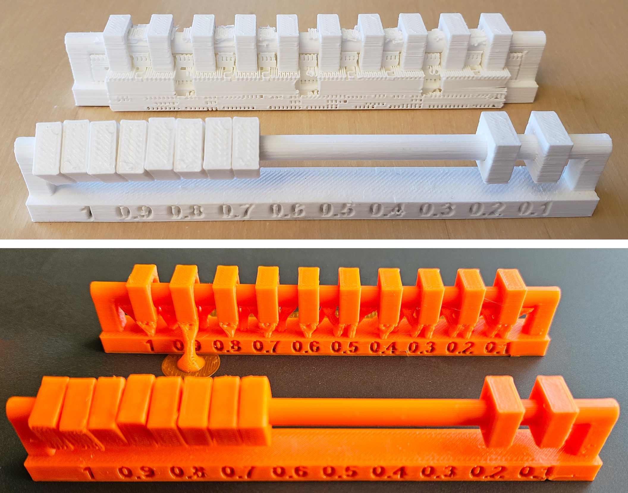
Group assignment: test the design rules for your printer. Below are the results from two printers at Waag.

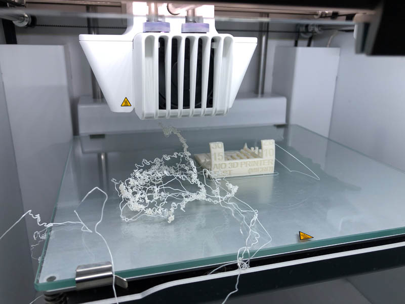
I also tested the design rules of the Ultimaker S3. And of course no Fab Academy 3D printing week without spaghetti! The second model came out nicely.

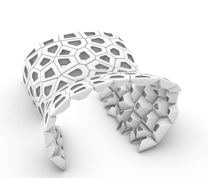
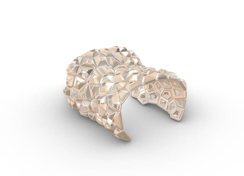
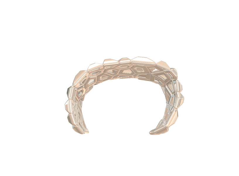
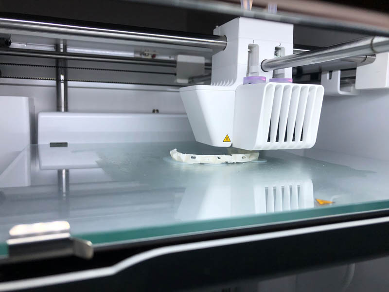
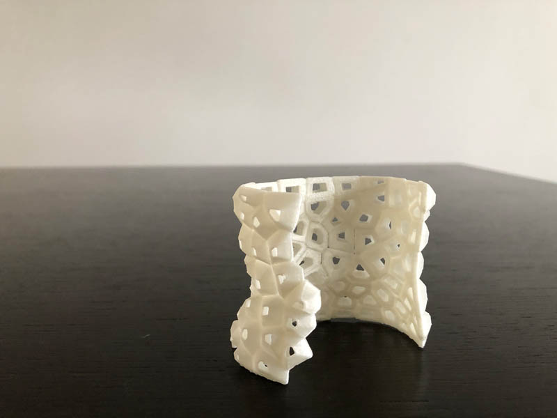
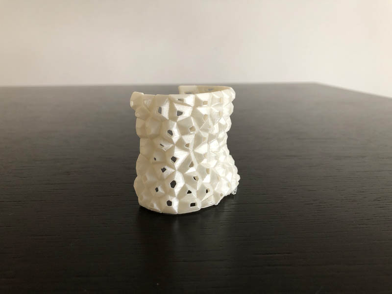
3D printing: nature-inspired bracelet, parametrically designed in Rhino and Grasshopper.

3D scanning: a comparison between four types of software applications and hardware: 3D Sense, 3DsizeME, Skanekt and the Qlone app. Conclusion, 3D scanning is not quite there yet.

How-to’s are below!

Back to top

Group assignment

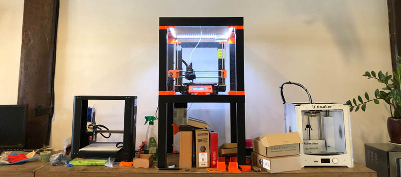
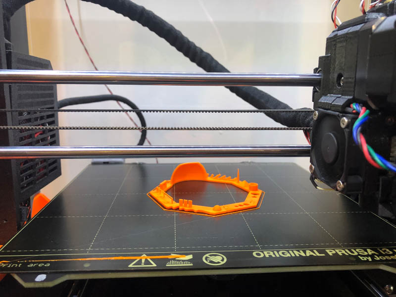
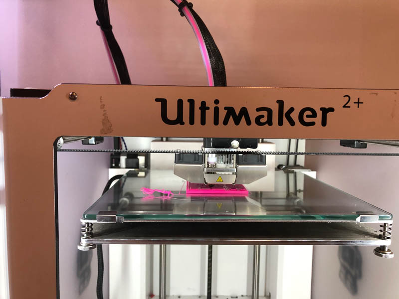
The 3D printers at Waag we’ll be working with are the Prusa i3 MK3S (middle) and the Ultimaker 2+ (right). In addition, I’m also going to find out what the design rules are of the 3D printer at home, an Ultimaker S3.

Prusa i3 MK3S

At Waag, we divided tasks among the group. Nadieh and I tested the Prusa. This is a really cool machine because it’s partly 3D printed with the Prusa i3 MK3 ENCLOSURE available on Thingiverse. We decided to go for the Test Your 3D Printer! model, also from Thingiverse. A day earlier, Douwe and Paula tested the same model on the Ultimaker 2+. By duplicating their exact settings, we would create two identical prints that can be compared.

First, we uploaded the .stl file in PrusaSlicer, the open-source software tool developed by Prusa. We set the Print settings to a resolution of 0.15mm QUALITY, Filament to Prusament PLA, Supports set to None, and applied an Infill of 30%.

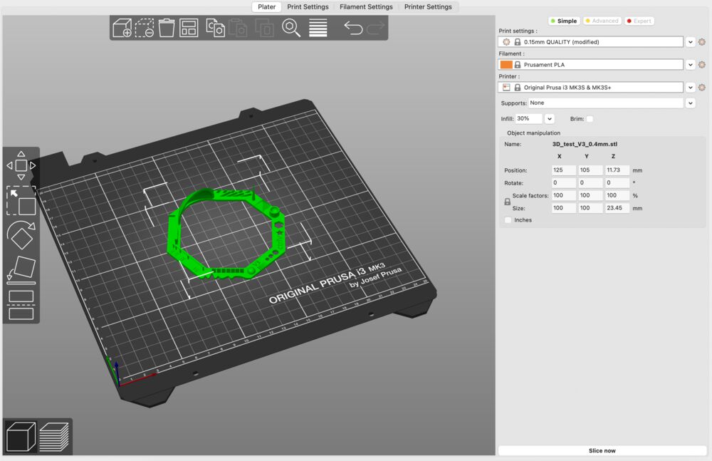
Then we sliced it by hitting the button in the bottom right corner, and saved the .gcode to the SD-card of the Prusa.

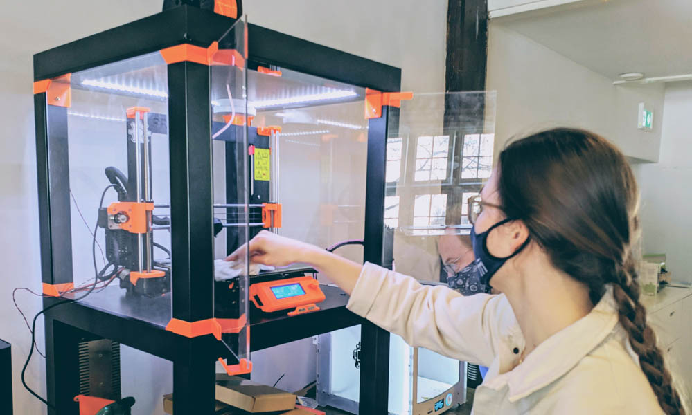
The next step is to make sure the printing bed is clean. It is necessary to remove grease for successful adhesion. We used window cleaner and paper towel.

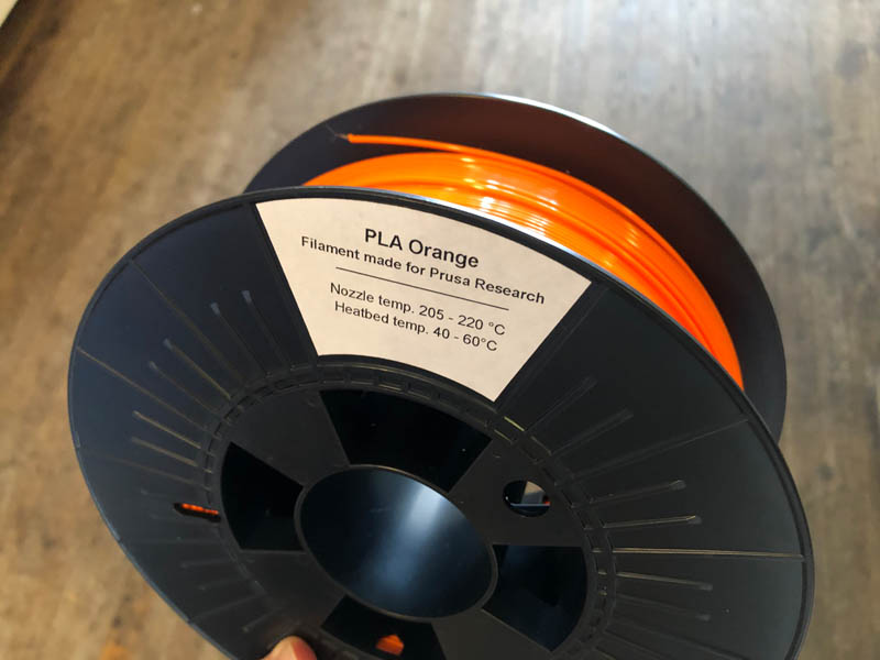
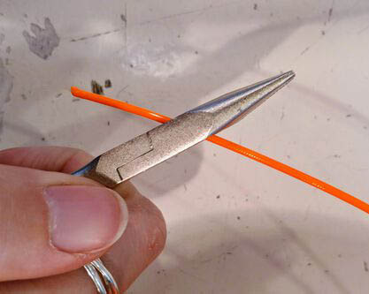
The filament we used was PLA Orange. When printing with this material, the nozzle temperature should be 205-220 °C and the heated bed temperature 40-60 °C. We learned a useful trick to cut the end of the filament at an angle of 45°. This eases the loading process.

The Prusa at Waag is programmed to unload its filament after each print. This is useful, because at a Fab Lab machines are continuously used by different makers, each with their specific material preferences. That’s why we start with loading the filament.

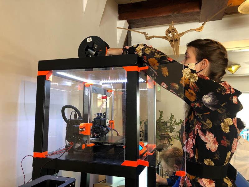
In contrast to the Ultimaker, where the filament spool is attached to the back of the printer, this Prusa has its spool holder on a rolling bed on top. You can push the filament down the tube until you feel resistance. The motor block on the printing core will pull it further down through the nozzle during the loading process.

Side note: that’s also different compared to an Ultimaker, where the engine is placed on the back of the printer, outside the enclosure of the printing bed. This results in a longer travel path for the engine to push the filament, which might make it more vulnerable.

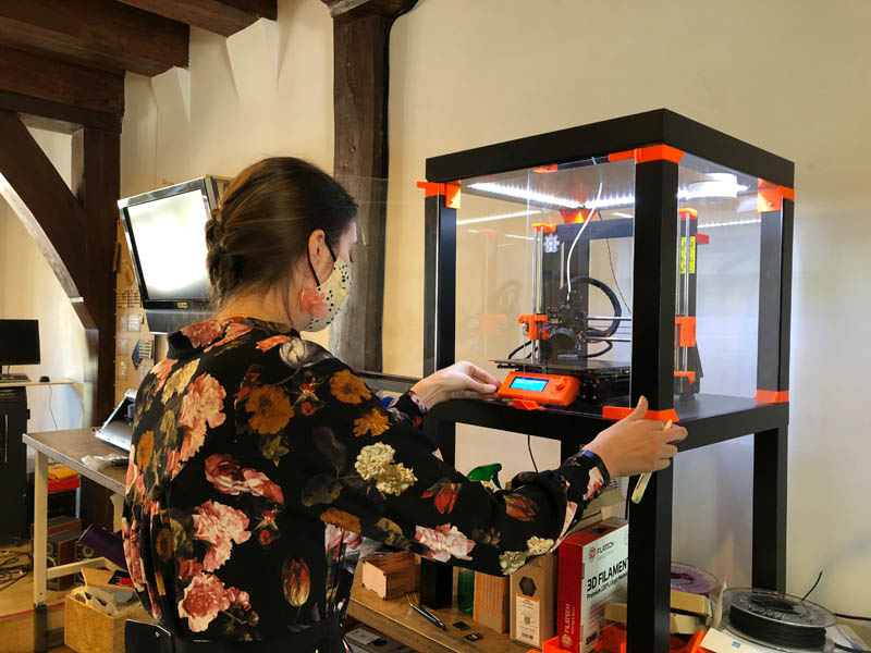
Now you can turn on the printer. The switch can be found on the backside of the back-left table leg. After that we inserted the SD-card.

When the printer is on, click Load Filament on the display, then select PLA - 215/60. It will start to preheat first.

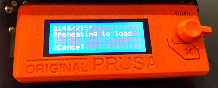
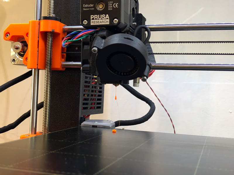
After a while, the extruder will spit out filament. When the nozzle extrudes a proper amount of material, you can stop the loading process. After that you can calibrate the printer.

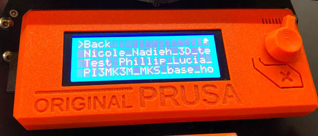
Then we opened our file. The standard printing speed was 150%. We changed this to 120%. The printing time was estimated at approximately an hour.

It is important to always check if the first few layers print correctly. That’s the most critical part of a successful print.

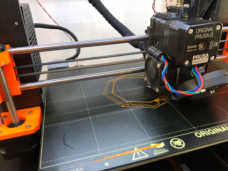
The model came out successfully!

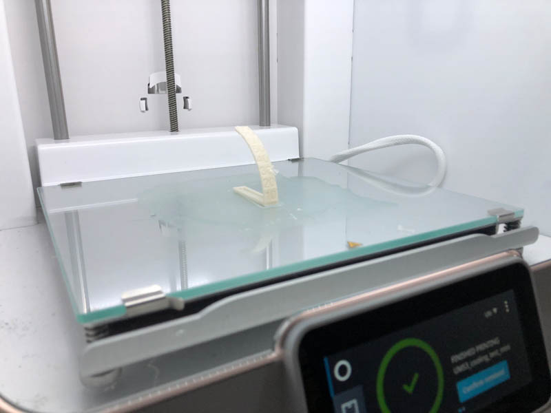
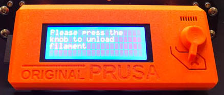
Now we can unload the filament. After the print finishes, Prusa will prompt this message.

After unloading, the Prusa asked us to load a new color. This is not what we were expecting. It turned out there were a few missing layers. As Nadieh describes:

I had already closed my PrusaSlicer file to inspect what I had done wrong sadly. However, after some googling about adding color layers in the PrusaSlicer, I saw how easy it is to add this, and how easy it is to miss as a new user (I described this already in the Preparing a Design for 3D Printing section). I think I must’ve probably accidentally clicked the little plus icon while dragging through the slices that added a new color (>﹏<) Thankfully it only happened at the very top of the design.

It was a good lesson! We decided that the print was good enough to be compared to the result from the Ultimaker 2+ printed by the other group. This is a picture of a different model on the Ultimaker 2+.

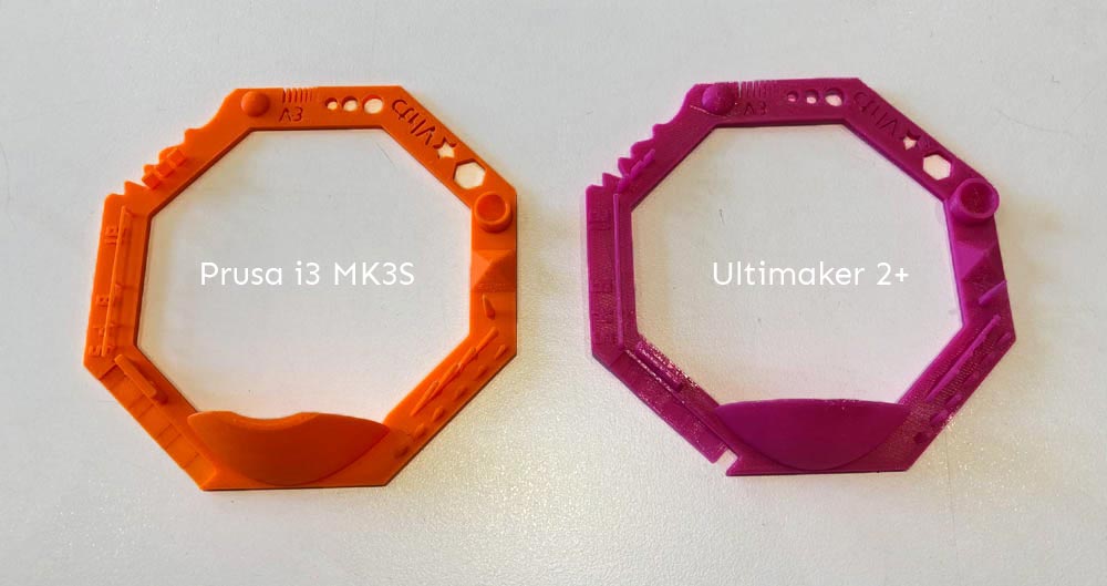
Here’s the comparison:

Detailed view: the Prusa generates a much smoother result at a higher resolution.

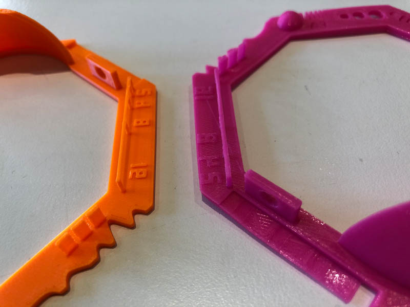
This is where you can see our little mistake ;-)

Back to top

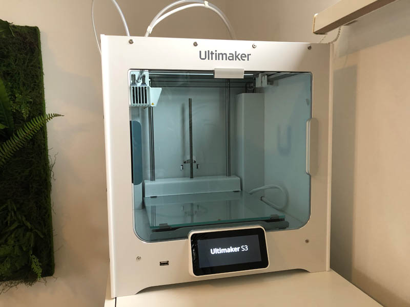
Ultimaker S3

In addition to the printers at Waag, I also checked the design rules of the 3D printer at home: an Ultimaker S3.

Print 1: MICRO All In One 3D printer test

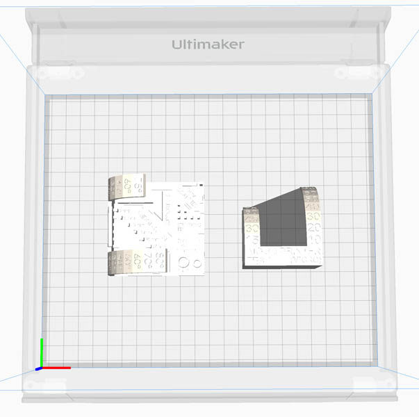
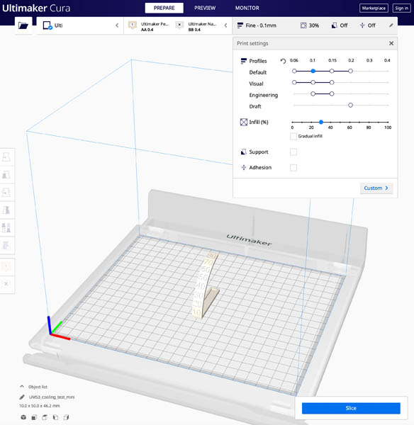
The user interface of the Cura software is presented below. I downloaded the MINI All In One 3D printer test from Thingiverse and imported it.

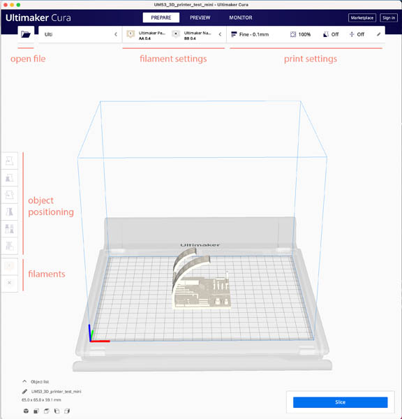
With the following settings:

• Profile: 0.1 mm (fine)
• Infill: 100%
• Support: no
• Adhesion: no

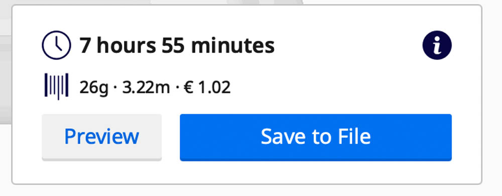
Click “Slice” to find out how long it takes to print.

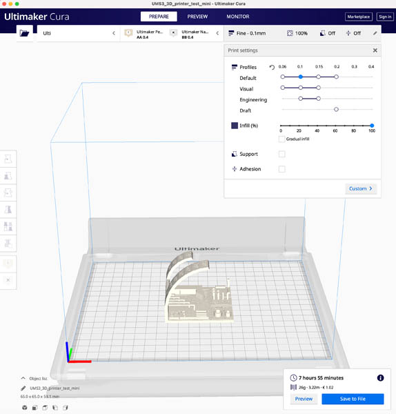
This would take way too long.

That’s why I continued searching, and found the Thingiverse MICRO All In One 3D printer test. This is a newer and more efficient model. It’s also smaller.

Rotate the model with the Snap Rotaton tool.

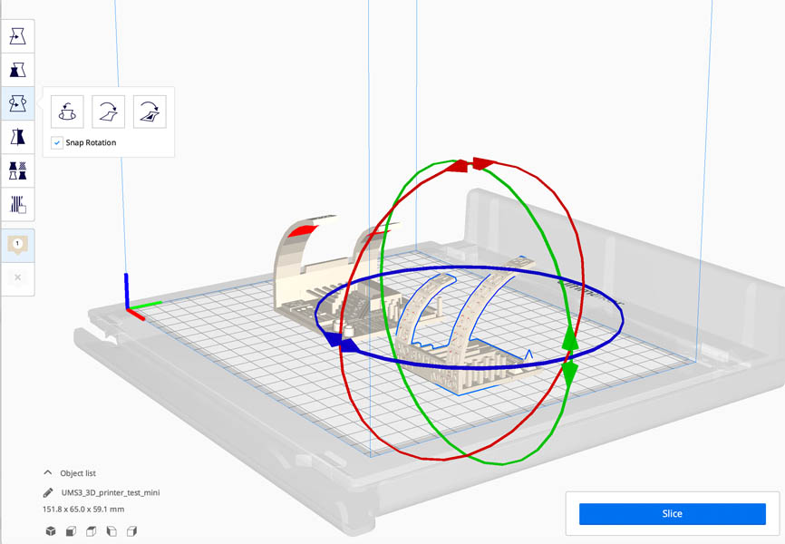
This model takes less time to print. But 4 hours and 27 minutes is still too long for me.

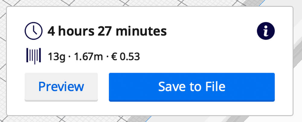
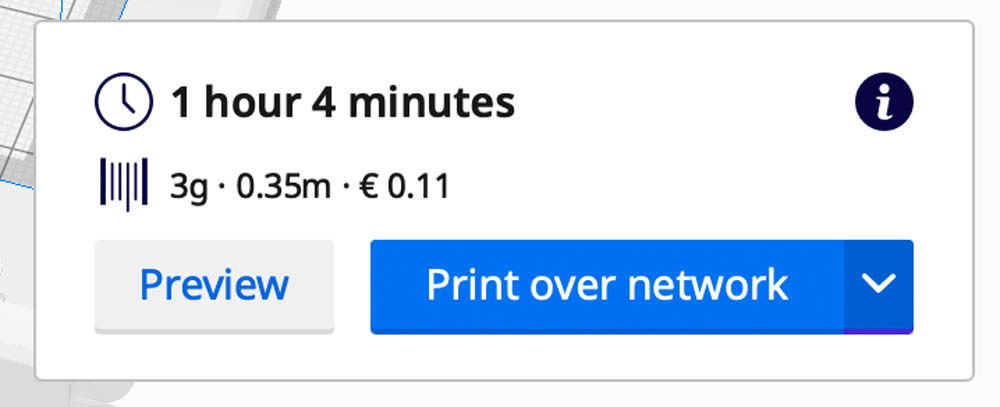
That’s why I changed the settings, as can be seen below. With an infill of 30% the print takes 4 hours and 14 minutes. It uses 13 grams of material, corresponding to 1.59 meters of filament.

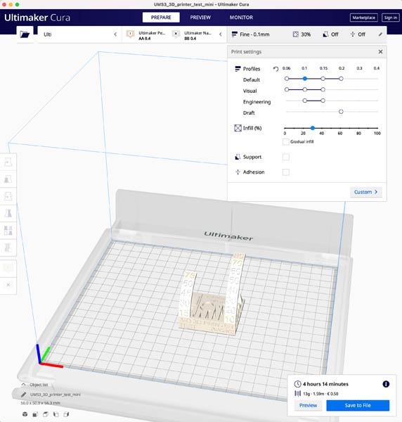
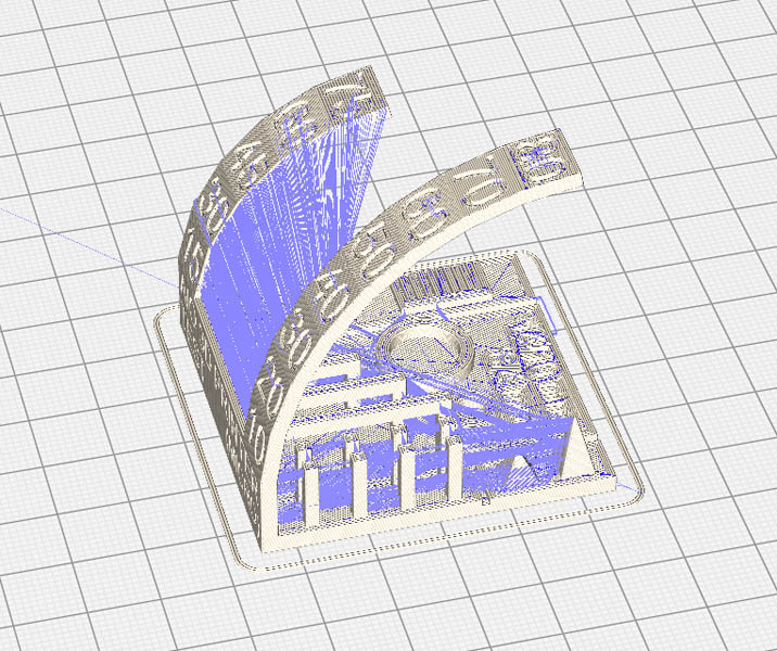
Preview the file by clicking Preview in the top navigation bar.

This is what the model looks like. It’s the path of the 3D printer.

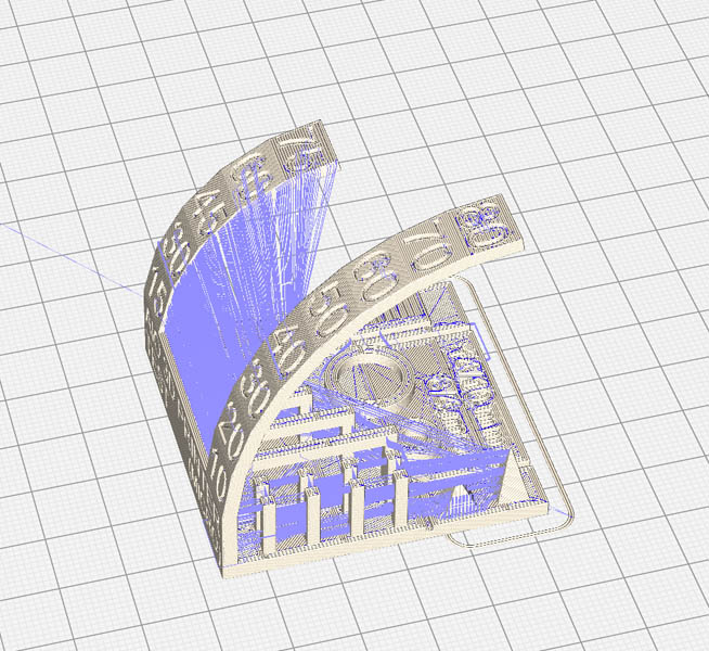
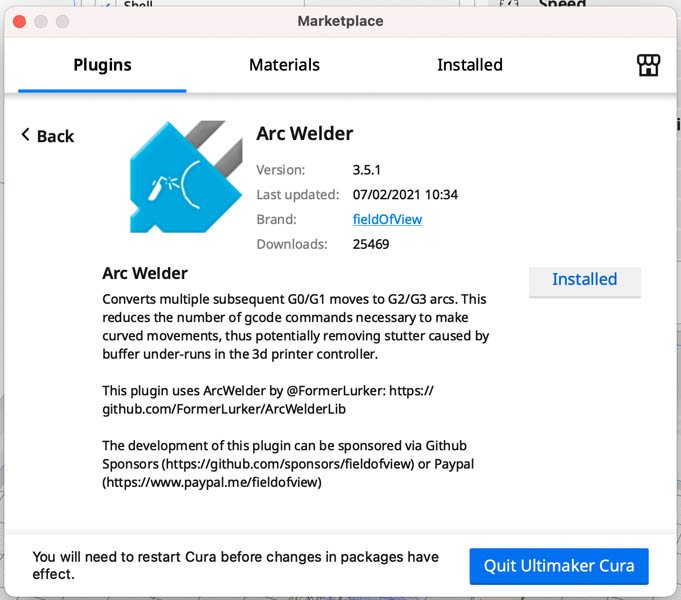
I want to see what happens with the Arc Welder tool. At the Ultimaker Marketplace, this plugin is available. I downloaded the Arc Welder tool, to test if the gcode can be optimized.

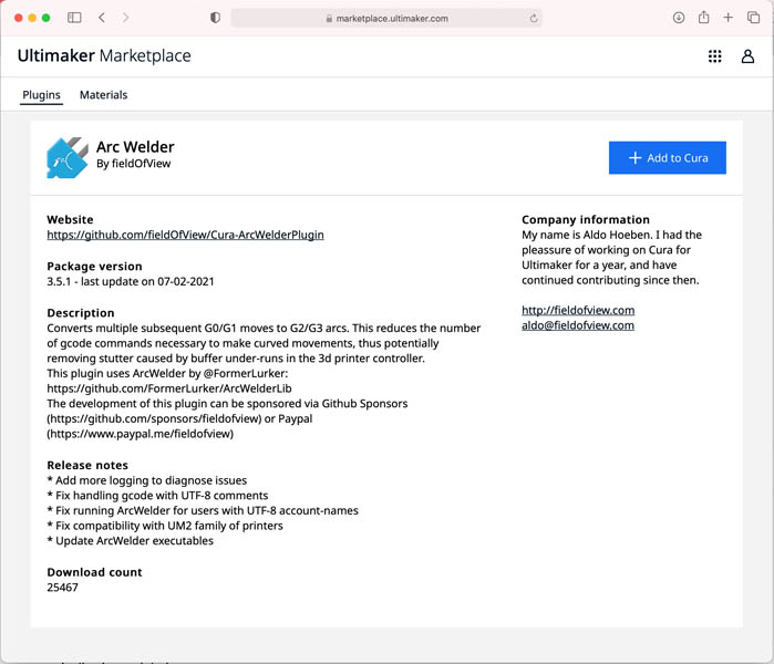
This is a description of what the tool aims to do:

After installation, I reopened Cura and the file. In Print Settings > Custom, Special Modes you can find the Arc Welder plugin.

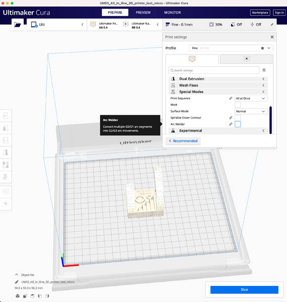
This is where you can enable Arc Welder.

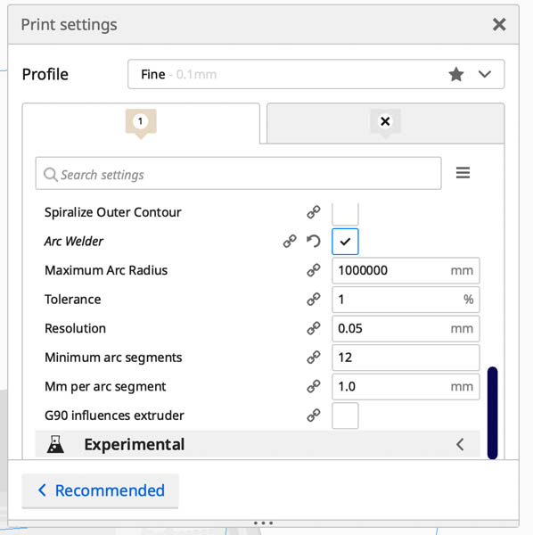
I kept the preset and sliced again. This is the new printing path. This is what the preview looks like:

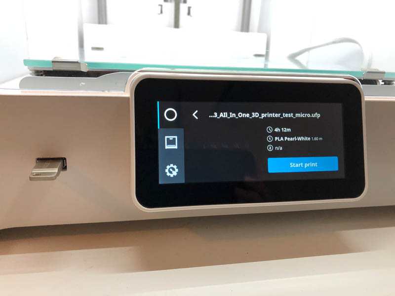
This yields a printing time of 4 hours and 12 minutes. It is a reduction of 2 minutes. It uses 13 grams of material, corresponding to 1.60 meters of filament. The Arc Welder tool reduces the printing time just a little bit. That’s certainly less than I expected. Because I want to print with a high resolution (Fine 0.1 mm) I’m ok with 4 hours printing time.

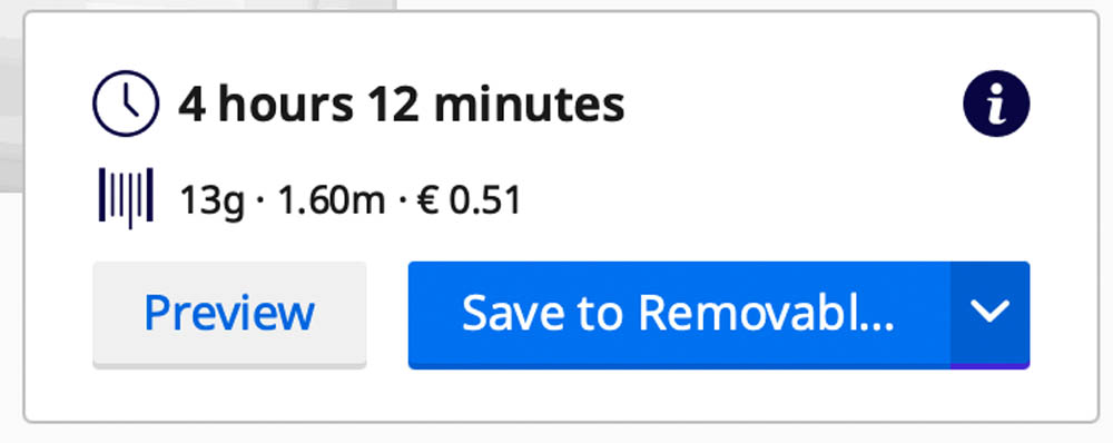
Next, you can upload the gcode on the removable drive. Cura’s interface is pretty intuitive and easy to work with.

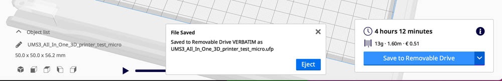
Now we can add the file to the printer. Use the USB port on front.

Select the file from USB.

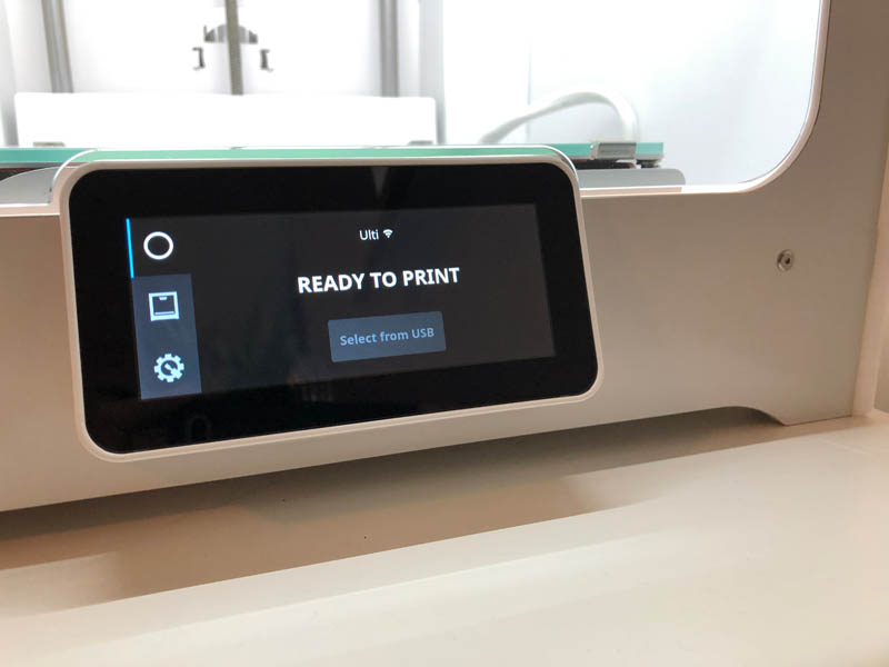
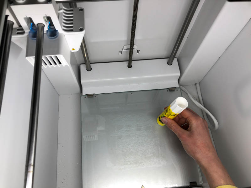
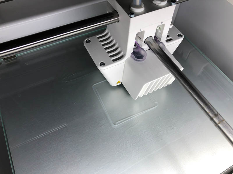
No, you’re not. We need to glue the build plate first! This is VERY IMPORTANT otherwise your design will stick to the build plate. At least, this is what I learned in the CBA fablab a couple of years ago. At Waag, nobody uses a glue stick.

Then open the file.

Ultimaker will heat up the plate and nozzle.

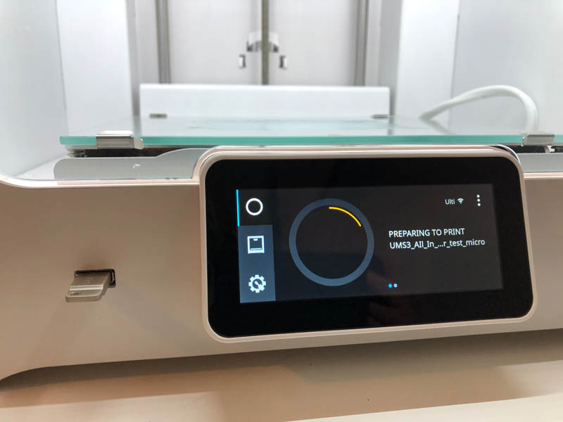
And starts printing the first layer. This is the most important layer.

FAIL! I suspect that this could be due to the path, that moves layer-by-layer from one overhang to the other. It doesn’t finish one overhang first.

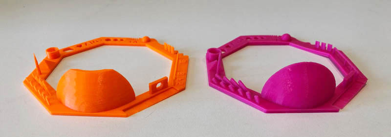
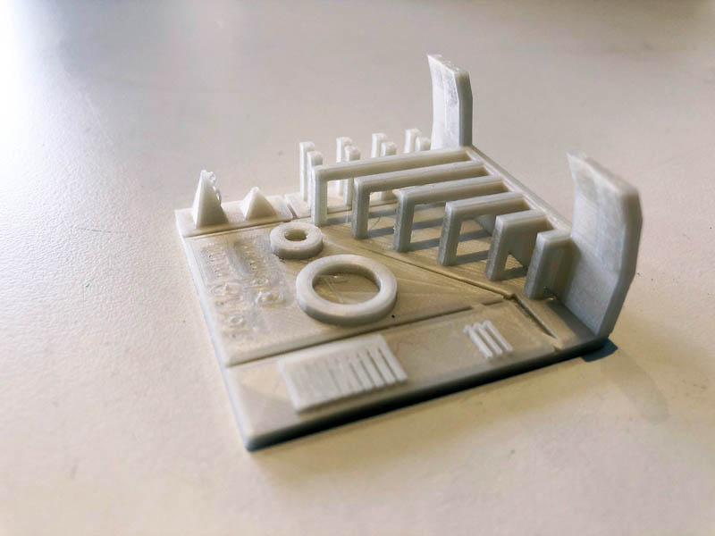
Results of this test:

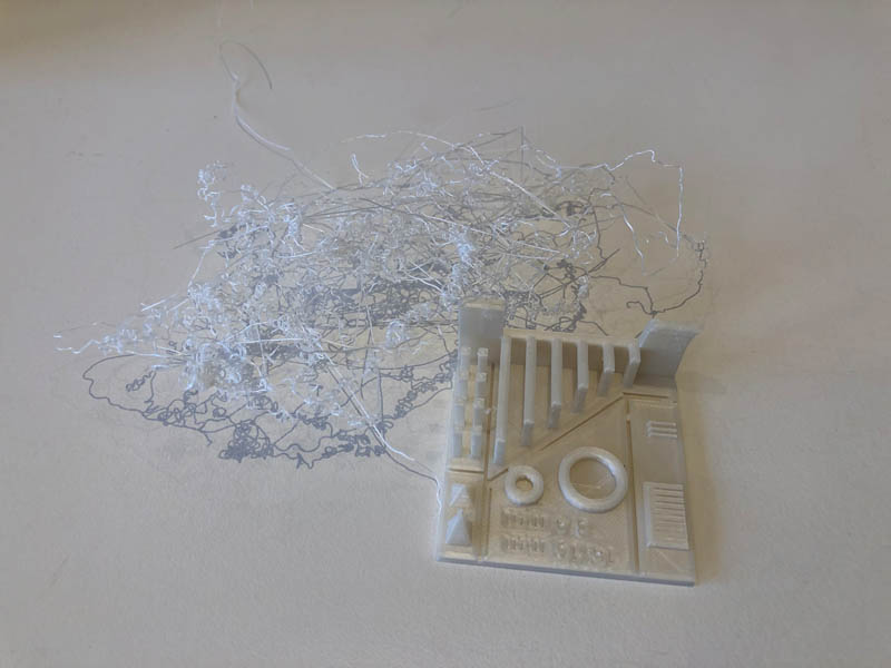
Still, I’m really impressed by the bridges. Prior to this 3D printing week I did not know of the possibility to print structures like this without support. That’s a major game changer for future designs! And it makes me really happy because it reduces material consumption and waste.

Print 2: Mini Cooling Test

Because the first model pretty much failed, I went on with a simpler model. The Mini Cooling Test is a remake, also available on Thingiverse.

You can follow your print on mobile with the Ultimaker app.

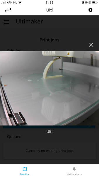
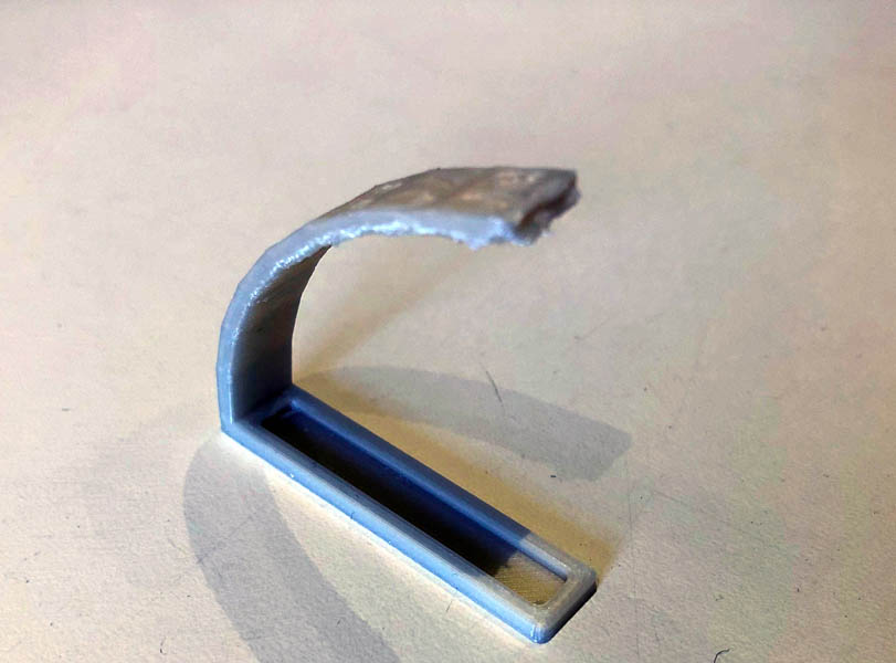
That looks a lot better!

The result: a beautiful overhang. I’m very impressed by the possibility to print without support and will incorporate this in my future work.

Back to top

3D printing

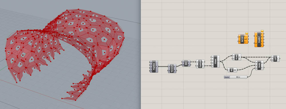
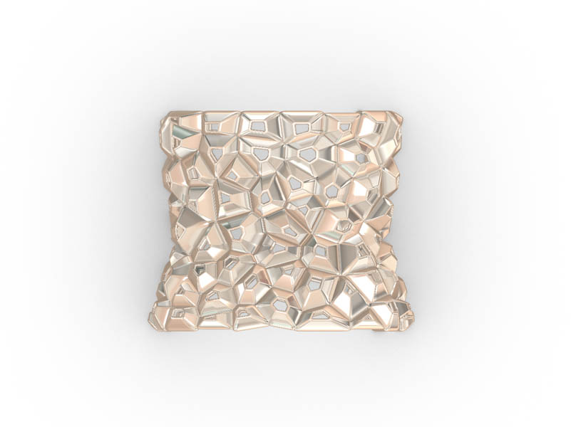
My inspiration for this assignment is the voronoi tessellation pattern that occurs in nature. For example in leafs, giraffe’s fur, honeycombs and cracked mud. The Computational Jewelry: Making of a Voronoi based Custom Bracelet using Rhino and Grasshopper by Mostafa Alani was a resource I used as a guidance. Note: this video goes really fast. I spent a long time hitting pause, moving back and forth, trying to capture a Jedi move or hidden command used in a fraction of a second. It’s clearly made by an expert and I reverse-engineered a lot of the components. In the sections below I’m breaking down the design process in small steps. Another tutorial video I consulted for a design experiment was the Voronoi structure on any surface example. I ended up not using this.

Parametric design in Grasshopper

First, start out in Rhino and draw one polyline. Copy it multiple times and scale the lines for a curved geometry.

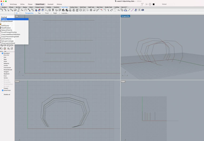
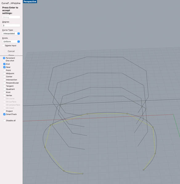
To smoothen the lines, use the CurveThroughPolyline command.

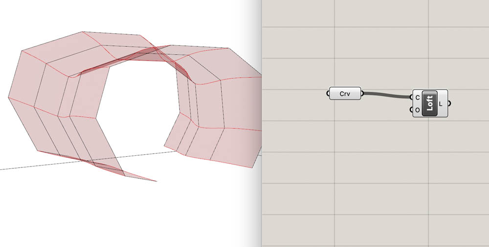
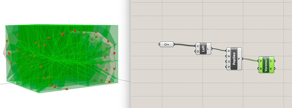
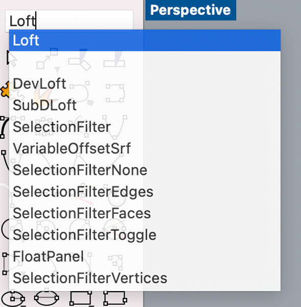
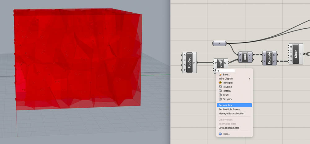
Then we open Grasshopper and link the curves. Type Curve to create the component, right click and select Set one Curve from the dropdown menu. Create a Loft component and drag a connection between the two.

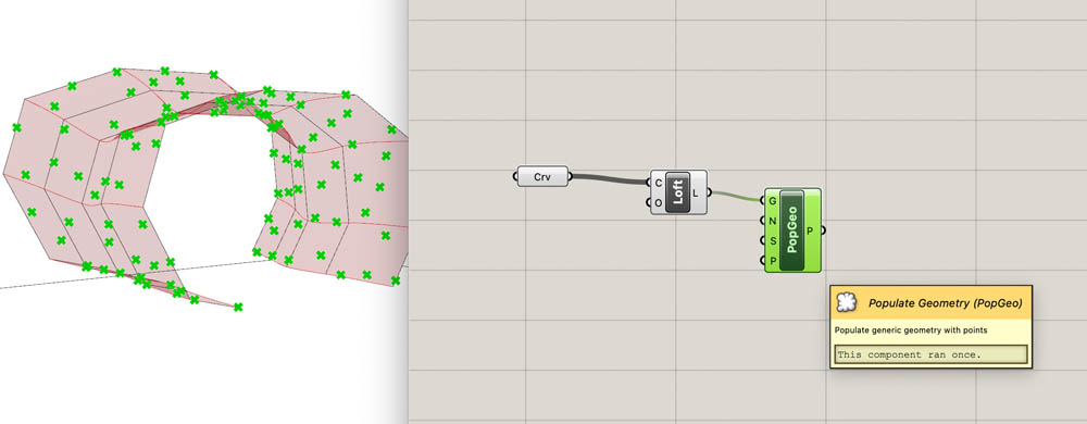
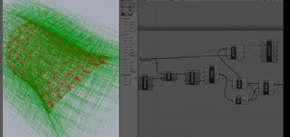
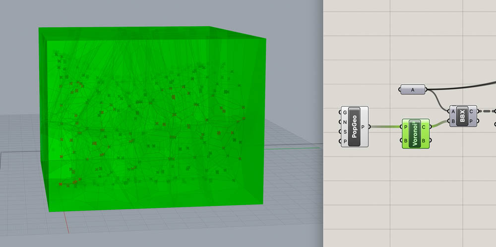
Now we add the Populate Geometry component. This creates points on the surface of the geometry.

Then add the Voronoi component. Drag a connection from the loft L to the geometry G in the PopGeo component. The B refers to a bounding box.

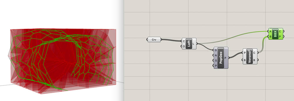
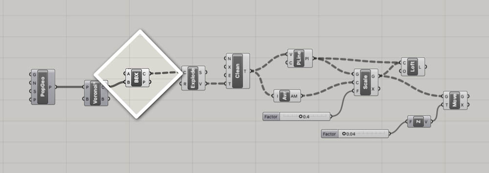
Now add the Brep BBX component. In short, a Brep is a boundary representation. This component solves intersection events for two input Breps A and B. Its outputs are intersection curves C and intersection points P.

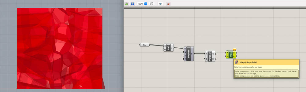
Connect the Loft component to input A of the BBX component and the Voronoi component’s C output to input B.

Add an Explode and Polyline component. Hide all components except PLine.

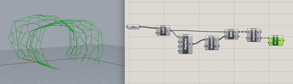
Connect Explode to Average. This places a point in the center of each geometry.

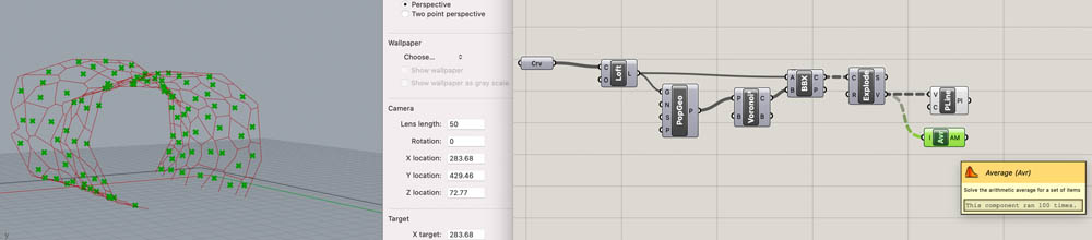
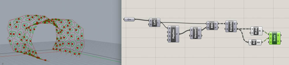
By adding a Scale component you can create a smaller or bigger copy of your geometry. Connect the Polyline to the geometry G input value of Scale and the output of Average to the input C of Scale.

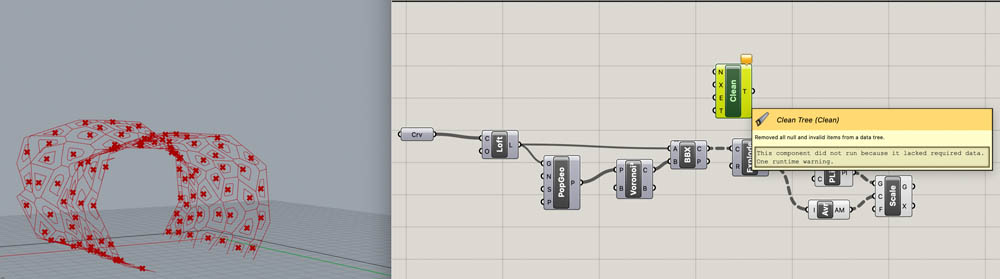
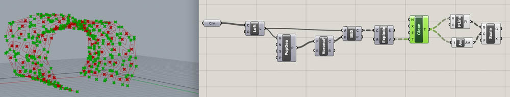
Next, add a Clean Tree component. I don’t know what this is, so I consulted the Delft University wiki on Grasshopper Data Tree Editing. They start with the following introduction:

Grasshopper uses, in contrast to a programming environment, no object names to define an object. This may sound trivial but it is one of the most fundamental differences from a traditional modelling environment. In Grasshopper the object or objects are placed in a list. The different lists of data are organized in a data tree structure where every branch and data content of the branch have an index number. Accessing the object is therefore more problematic than in a scripting environment. Grasshopper has various tools to remedy this problem. These tools supports the editing and selecting the content of the lists and editing the data tree structure. Knowledge of these techniques are essential for the effective use of Grasshopper.

They then provide a step-by-step explanation of how data trees work. The Delft University wiki is a great resource for understanding this better. If you want to dive deeper into this, I highly recommend reading this page.

We’re moving on to the design. Right-click on component Clean’s input values E, X and N to Set Boolean to True.

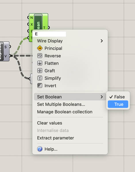
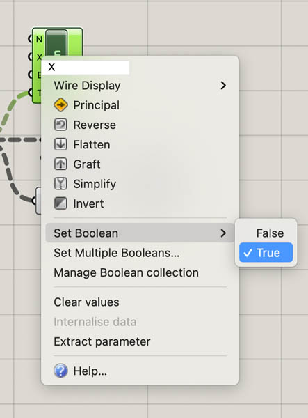
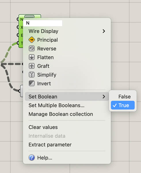
Then place the component in betwen Explode and Polyline and Average. Now the corner points of each geometry are activated.

Add a Loft component to create a surface in between the outer and inner geometry.

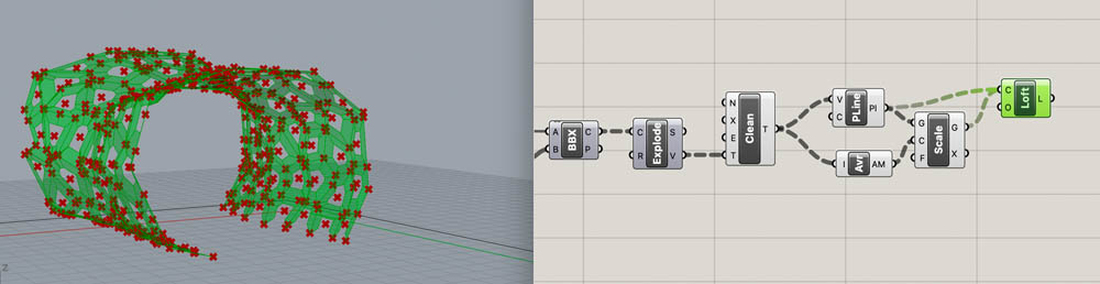
Then, add the Surface Closest Point and Evaluate Surface components to the canvas.

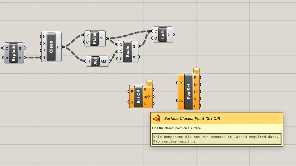
When I connected these components, it didn’t generate the expected result. I looked back into the canvas and found that the imported file from Rhino was not a Curve, but a Populate Geometry component. I initially didn’t use the direct input value of the Populate Geometry component because thought I could make this myself in Grasshopper with a Curve and Loft. So I went back and recreated the first step, which ended up working.

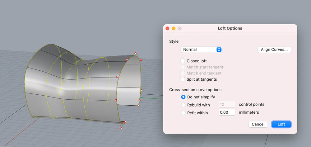
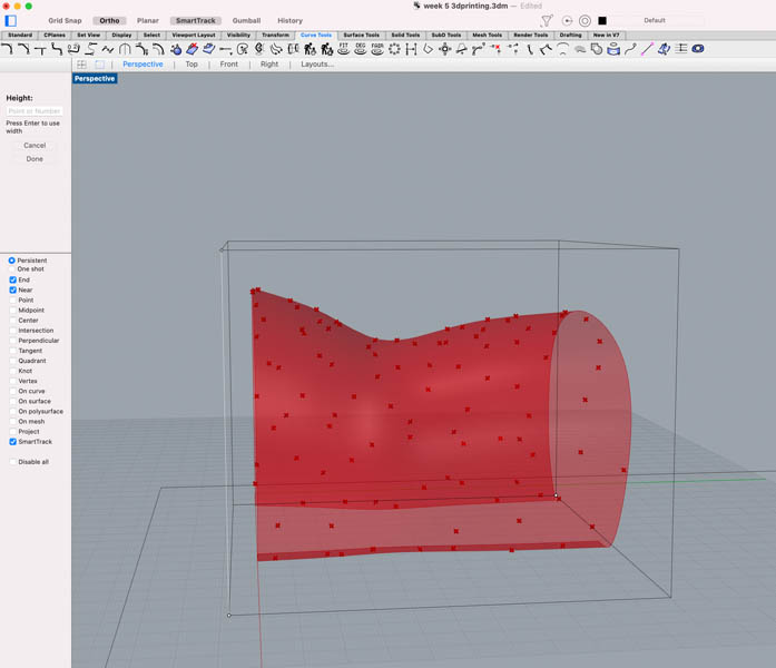
In Rhino, make a loft from the curves.

Settings at the pop-up menu.

Select the lofted shape in Rhino and create a Populate Geometry component in Grasshopper.

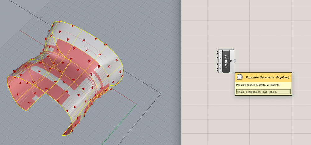
Connect it to the operations from before. That looks better! I also added a Number Slider to factor F of Scale to adjust the size of the internal geometry.

There was another item missing. Here, to be precise.

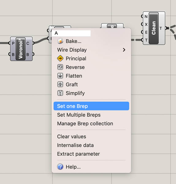
Right click on the A component and select Set one Brep.

Extract Parameter is a quick way of getting a parameter out of a component so that you can connect it to another component instead of attaching a panel or slider into it. This is also useful for sharing your design, because it internalizes the shapes created in Rhino. Right click A again and Extract Parameter.

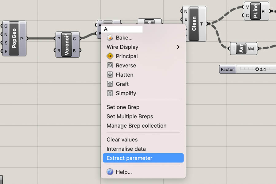
Then connect the extracted parameter A to Surface Closest Point and Evaluate Surface components. They are still orange because not all required input values are connected yet.

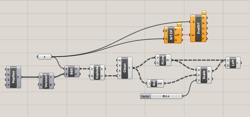
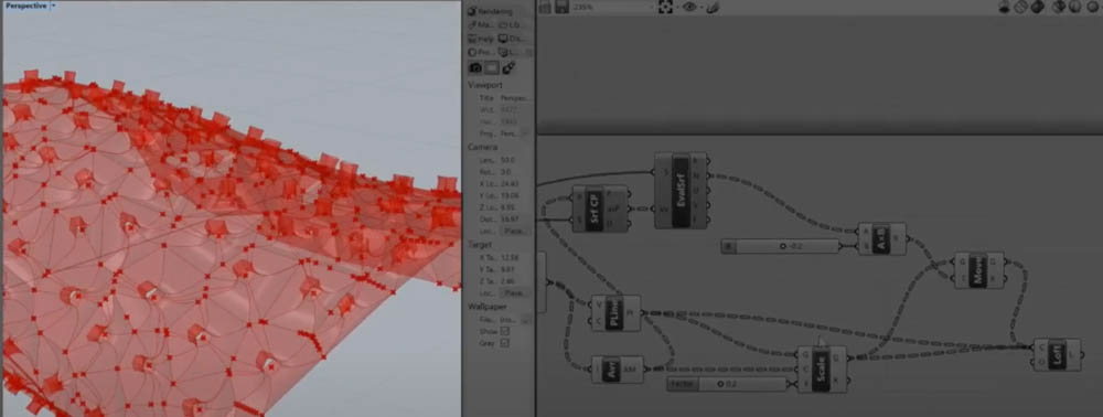
Connect the output of Average to the input P of Srf CP. Now the components run successfully without errors.

Now we add and connect two new components: Multiplication and Move.

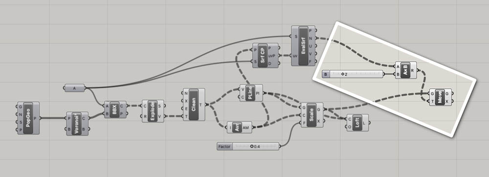
And add a number slider to the B input value of the Multiplication.

The Loft component creates a surface on this second layer.

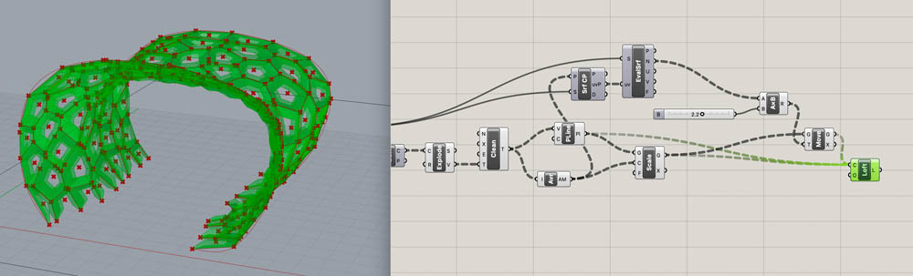
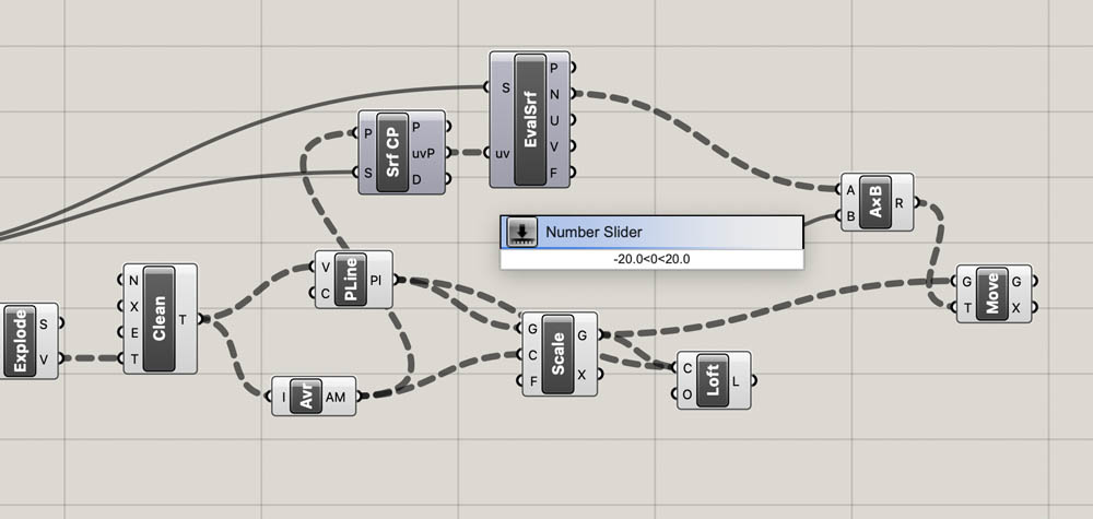
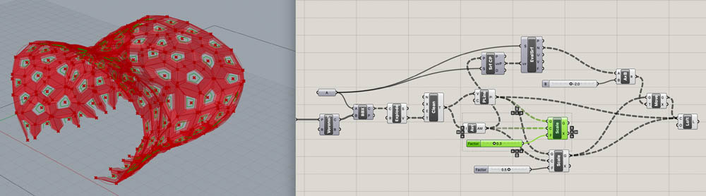
Add a number slider to the Scale component. The value below is set to 0.5.

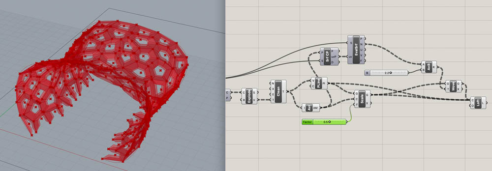
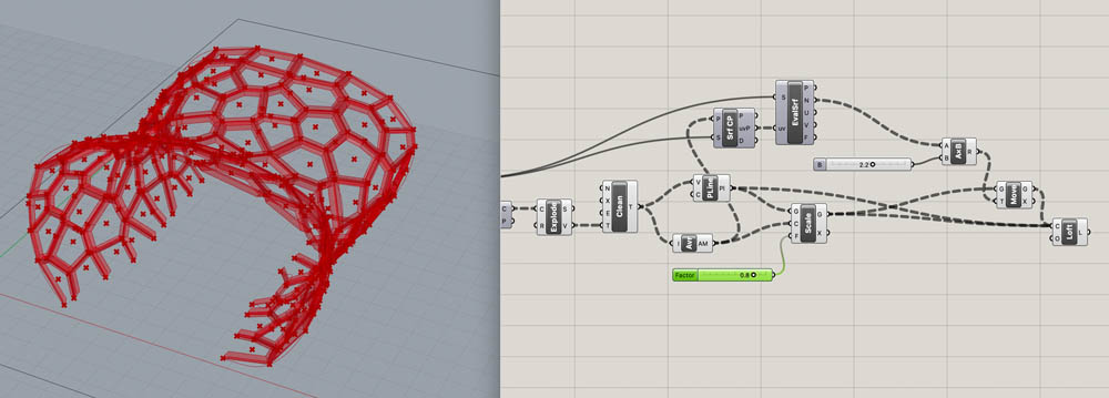
To illustrate, changing the value to 0.8 generates another structure.

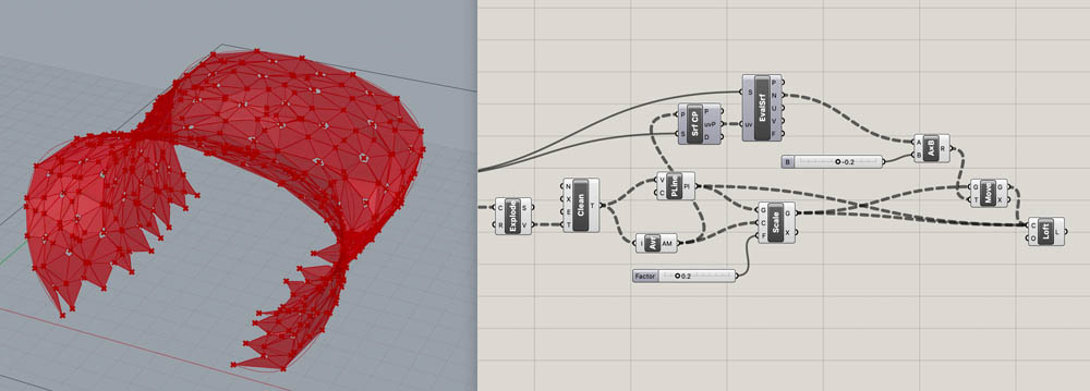
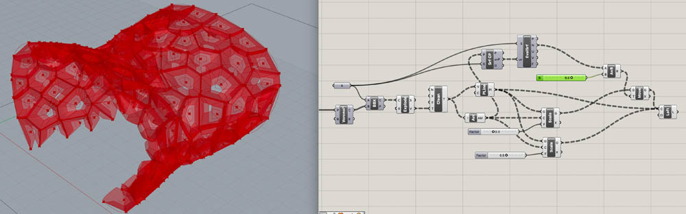
And changing the number slider to -0.2 creates even smaller openings.

The next step is to copy the Scale component. This is the beginning of creating a three-dimensional structure.

Connect the output geometry G of the newly added Scale component to Move.

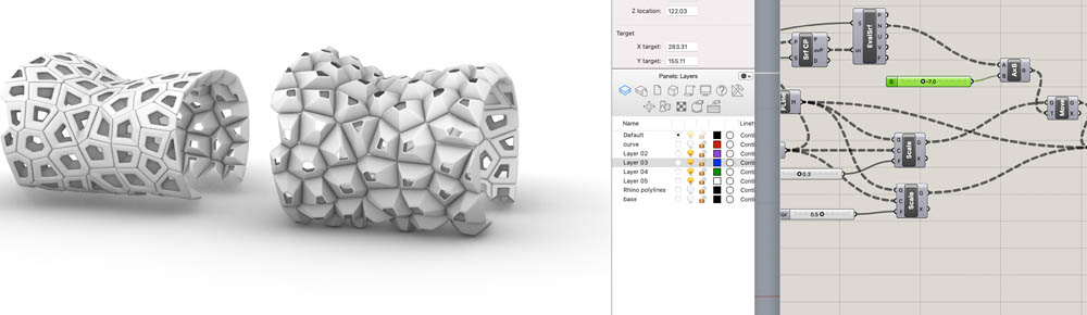
This is where I noticed another issue. My design doesn’t create the same shape as the tutorial, even though I replicated the grasshopper components precisely. The image below is a screenshot of the video.

I searched the Grasshopper and Rhino files to find the issue and decided to reconstruct the Grasshopper canvas from scratch. The moment the Average component is connected to the P of Surface Closest Point it should create pointy things, like in the screenshot of the video below. In my case, they are tiny. I suspect that this has something to do with the box that was set in Rhino.

On the Voronoi component, right click B and select Set One Box.

In Rhino, you can now draw the bounding box around your object by defining its width, length and height.

When you’re done, hit enter and the new bounding box appears. Because this box is further away, it creates longer lines. That’s exactly what we want!

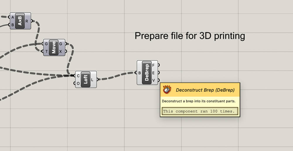
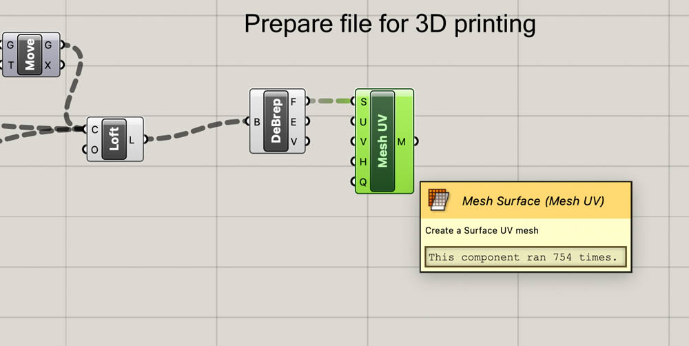
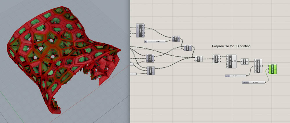
Now we can move on to prepare the file for 3D printing. To keep the file easily readable, I like to name the sections. This can be done with Scribble. To start with file preparation for 3D printing, add the Deconstruct Brep component.

Then add the Mesh Surface component.

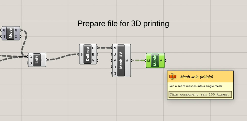
And join the set of meshes into a single mesh with Mesh Join.

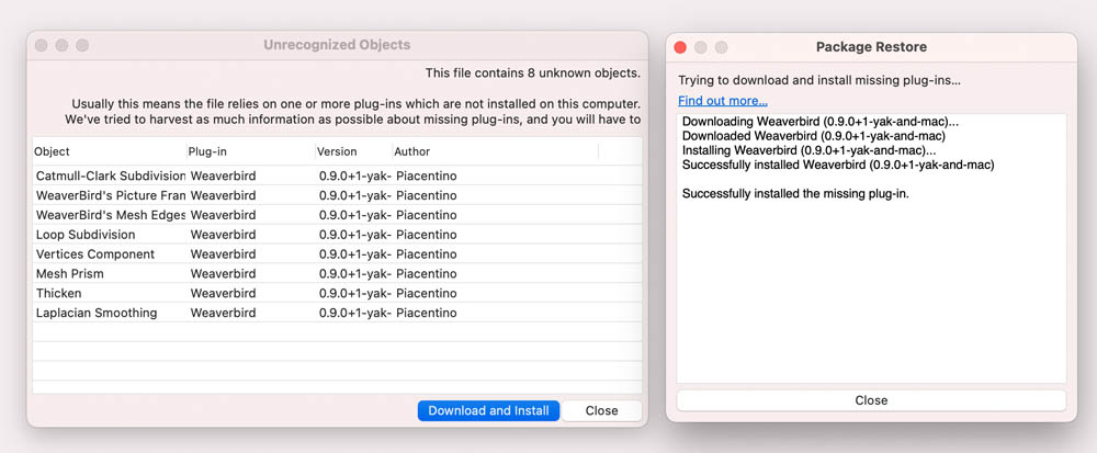
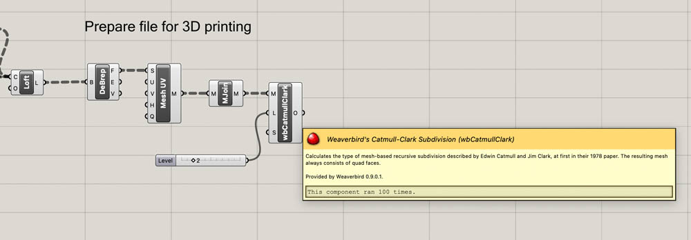
For preparing the file, we need the Weaverbird plugin for Grasshopper. You can download it here. This is a topological mesh editor. We need it for the Catmull-Clark Subdivision.

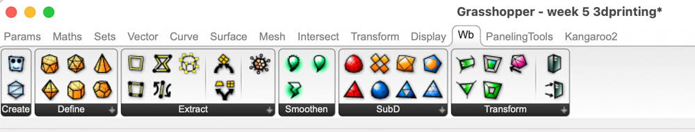
This is what the Weaverbird tab looks like in Grasshopper.

Add the wbCatmullClark component and link a number slider = 2 to input value L.

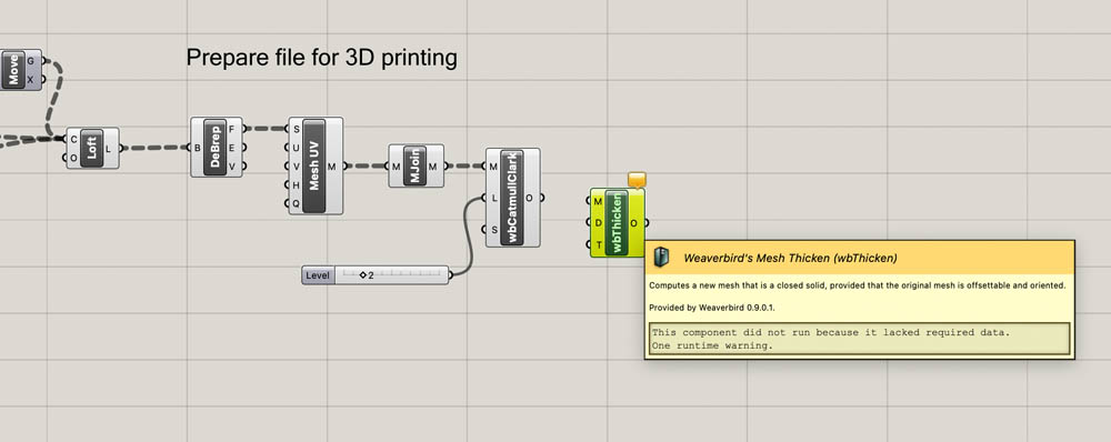
Then add Weaverbird's Mesh Thicken to compute a new mesh that is a closed solid.

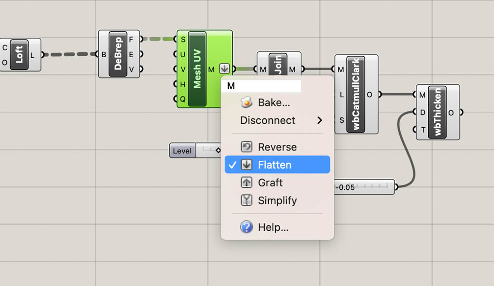
Right-click on the output value M of Mesh UV to Flatten the data.

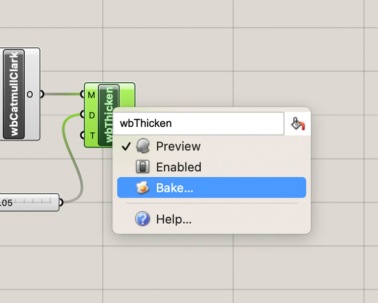
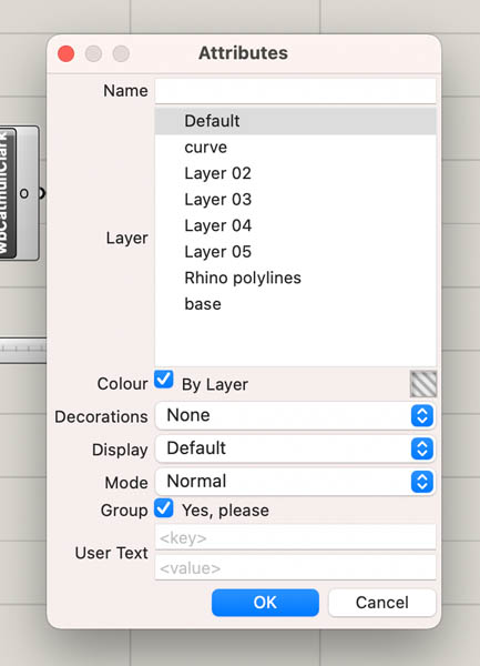
And right-click on Weaverbird's Mesh Thicken to bake the results in Rhino.

Choose a layer from the pop-up menu and check the Group box.

A duplicate of the file will be created in Rhino. Your Grasshopper file is also still there. You can hide the Grasshopper components.

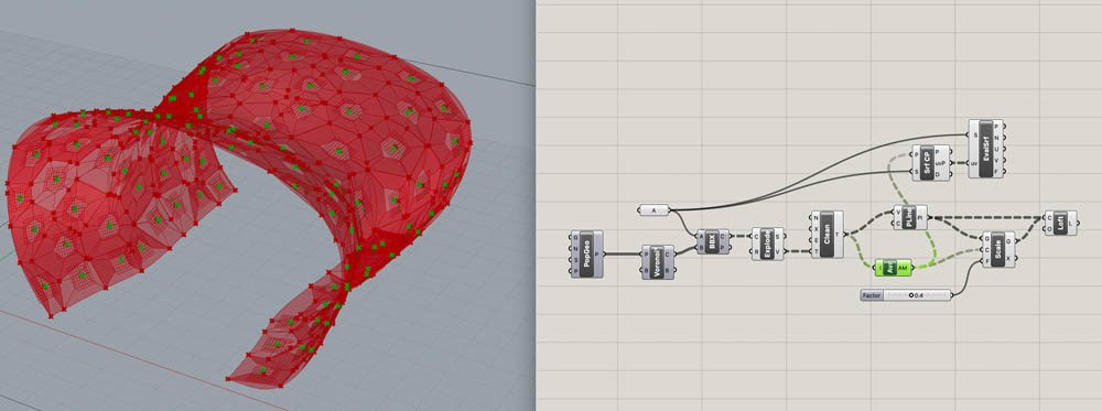
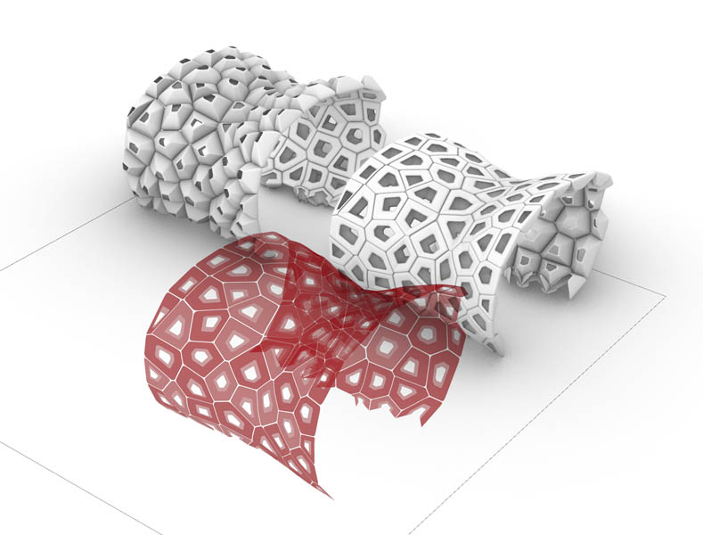
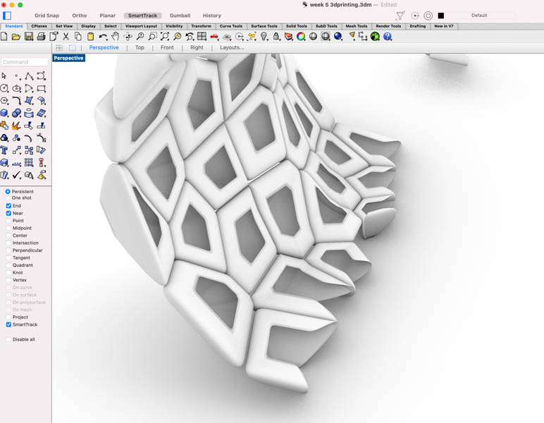
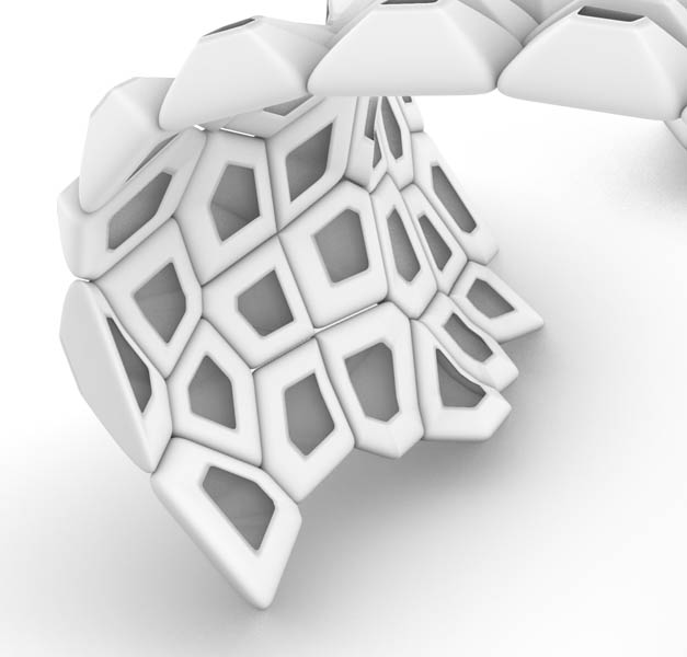
Set the Rhino view to ‘Render’ and.. BOOM!

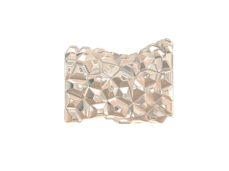
Plus an inverted version:

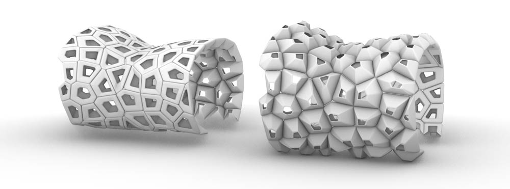
The inverted shape can be achieved by changing the slider in the AxB panel to -7.0.

Back to top

Post-processing design

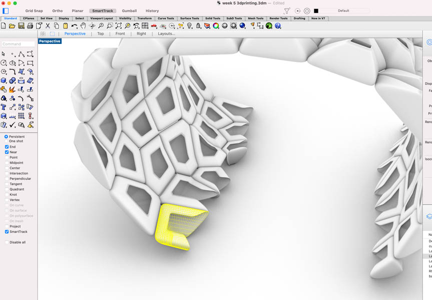
Some post-processing was needed, because I didn’t like the open edges that were created on the ends of the bracelet.

This is a close-up. You see? It’s so ugly!

Select the object in Rhino, type Ungroup in the command line and then Explode.

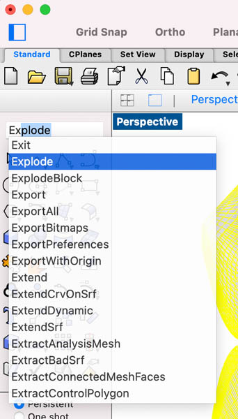
Now you can select each item individually, and delete them.

So much better <3

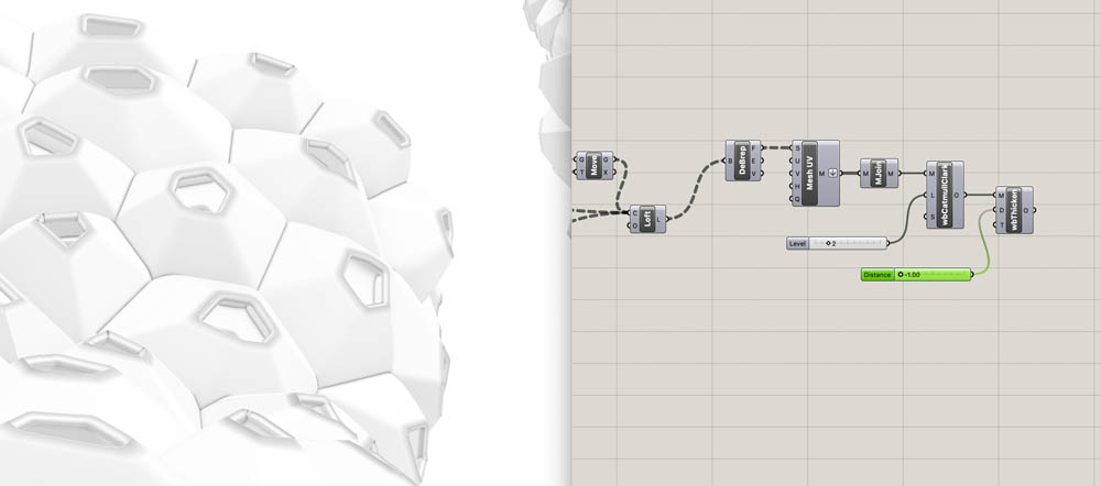
To increase the material thickness, I went back to Grasshopper and played with the distance slider of the Weaverbird's Mesh Thicken component.

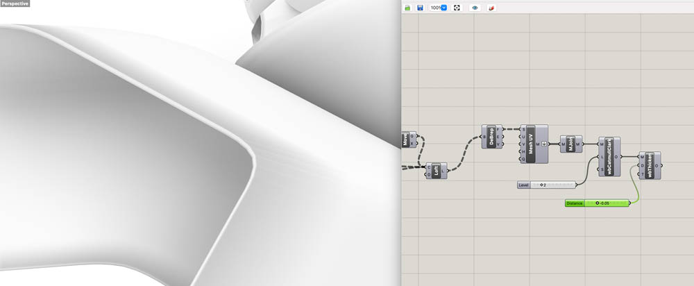
Here you see how the material thickness is adjusted when we change this from -0.05 to -1.00 mm.

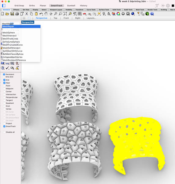
After this step, I baked in Rhino again, ungrouped and exploded the design to control each element individually, and deleted the ugly edges. Now we’re ready for some final post-processing before 3D printing. Select the geometry and type MeshRepair.

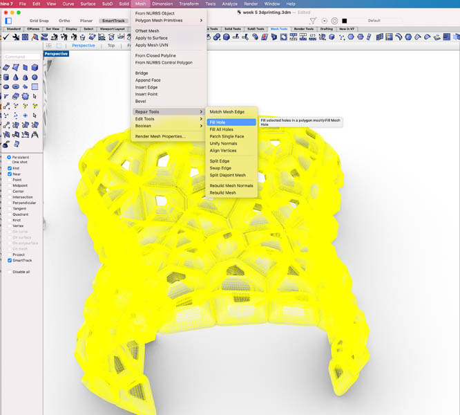
Then navigate to Mesh > Repair Tools and click Fill Hole.

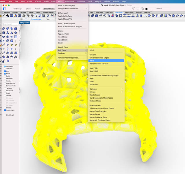
After this, do the same for Weld.

Now you’re ready to export the selected design as an .stl file and send it to the 3D printer.

Back to top

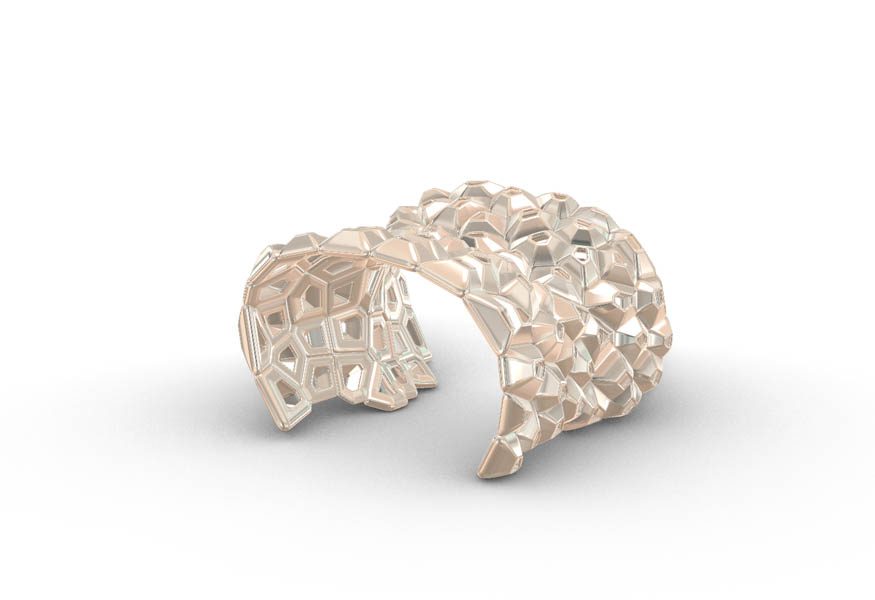
Rendering

If you want you can make a rendering of your design, like we learned during CAD week :)

3D printing

The first step is to import your file in the Ultimaker software.

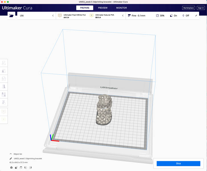
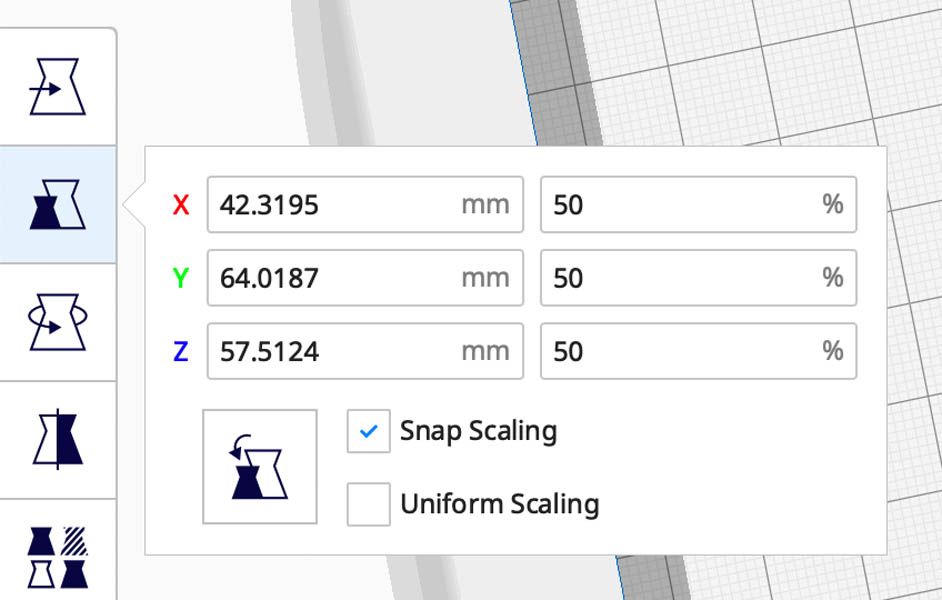
You can change the size of the bracelet here. I made it 50% smaller because I have a tiny wrist. The model itself is rather big.

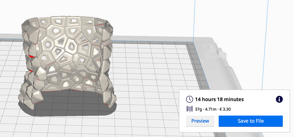
I clicked Slice to see what would happen if I would work with a profile of 0.06. Over 14 hours of printing time is way too long for this exercise.

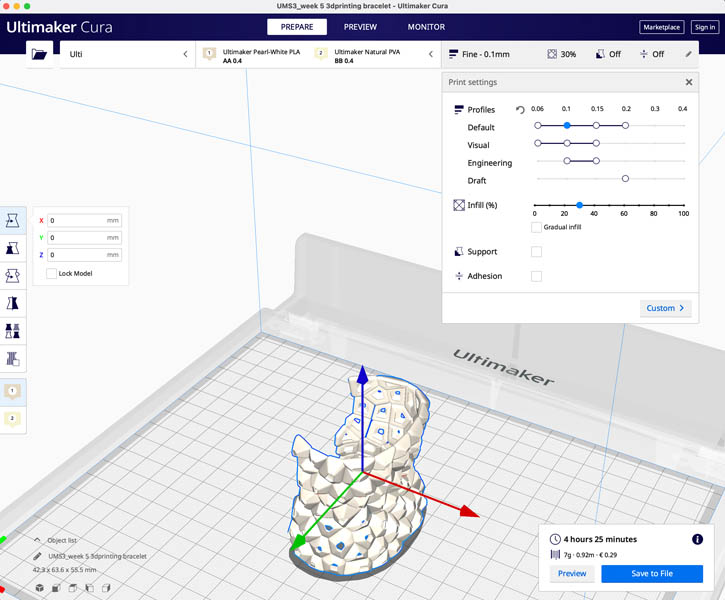
So I changed the profile to 0.1 and removed the support. The infill is set at 30%. After slicing, the estimated printing time is now 4 hours and 25 minutes.

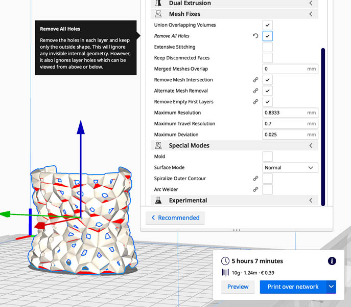
Next, experimented with more advanced settings to reduce printing time. For example, ‘remove all holes’. That actually increased the time to 5 hours and 7 minutes.

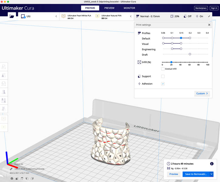
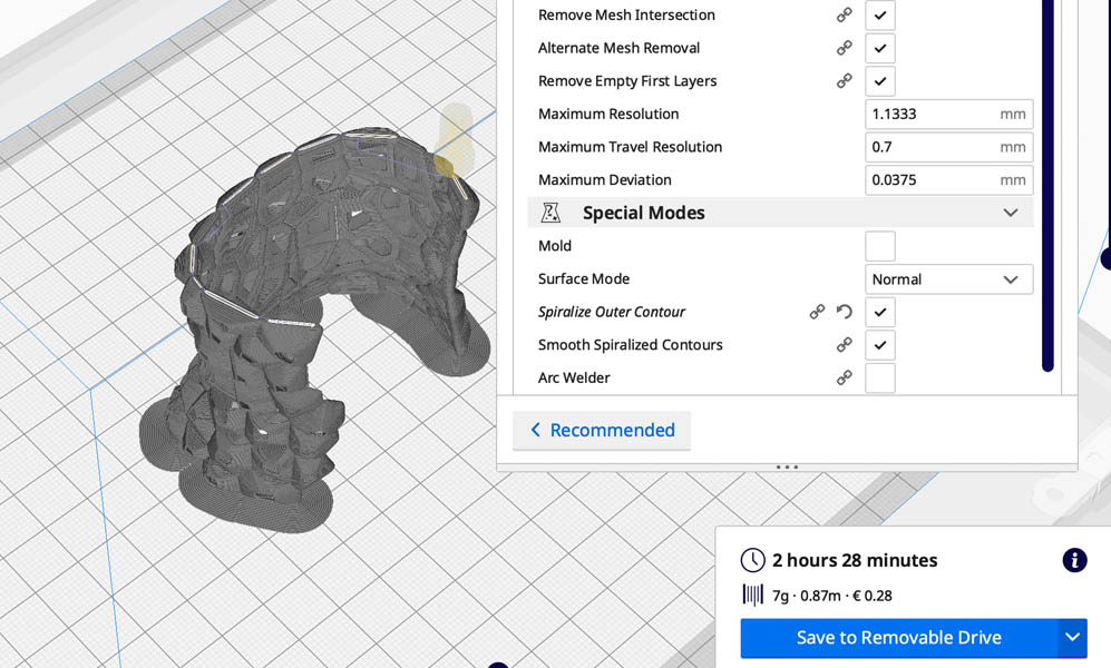
Then I increased the profile to 0.15 and reduced the infill to 20%.

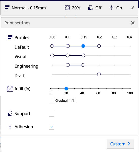
This resulted in a printing time of 2 hours and 49 minutes.

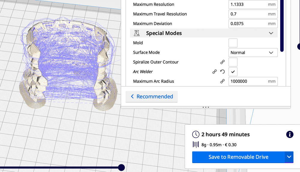
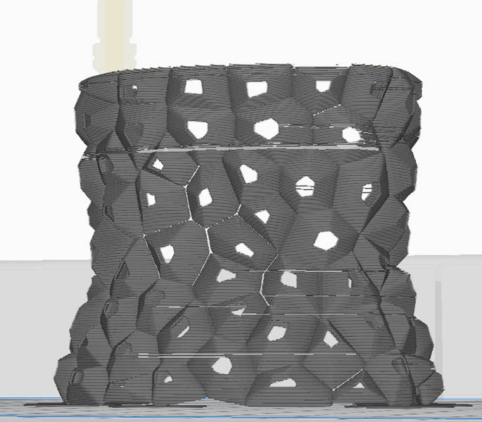
Then I tried to further reduce the printing time and material use with the Arc Welder plugin. The printing time remained the same, and the path doesn’t seem to be more efficient. As you can see, the purple lines still travel across the object, instead of creating a continuous path following the design.

I also tried the Spiralize Outer Contour functionality.

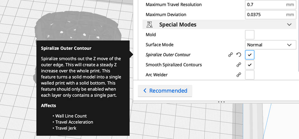
This resulted in a printing time reduction of only one minute.

And a closer inspection of the path doesn’t make me very happy.

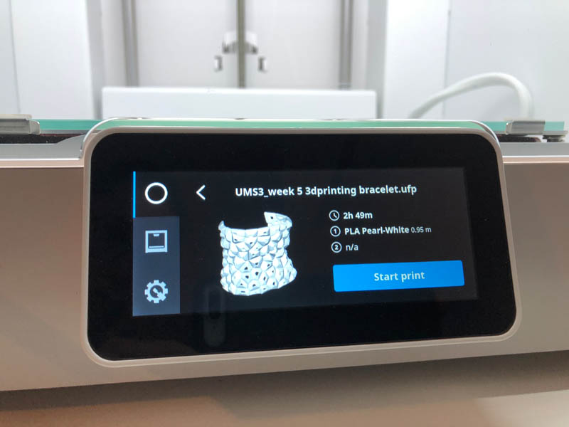
Therefore, I unchecked all special modes and went with original the printing time of 2 hours and 49 minutes. I exported the .ufp file on an USB and uploaded this on the Cura.

The first layers are always the most vulnerable. Make sure to stay close to the 3D printer during this initial phase, in case something goes wrong.

About halfway into the printing, and when the printer was ready.

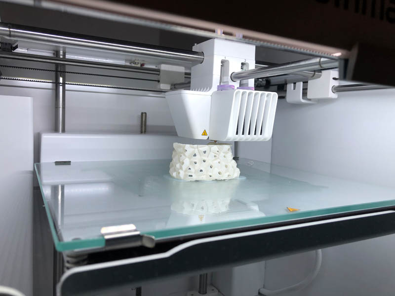
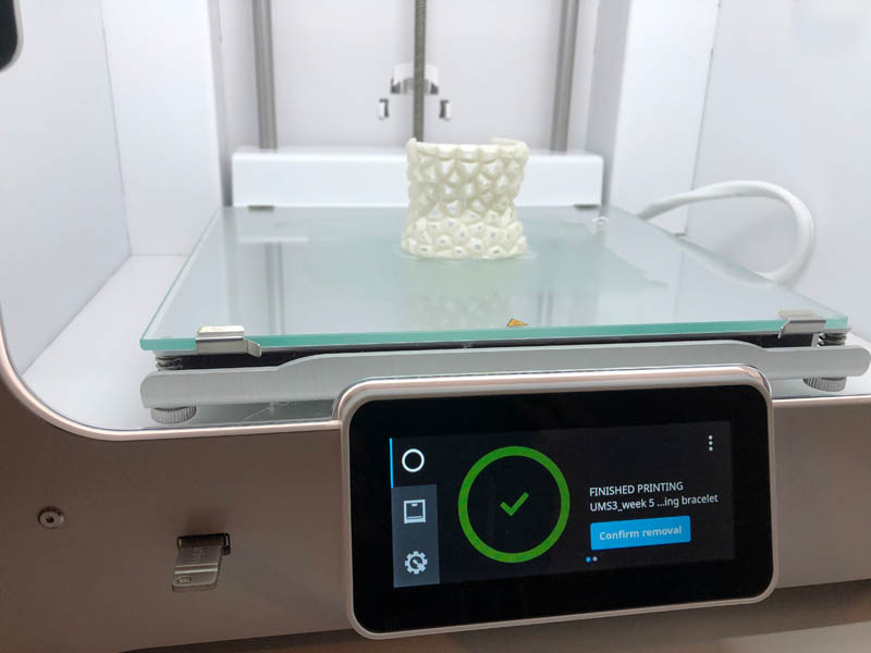
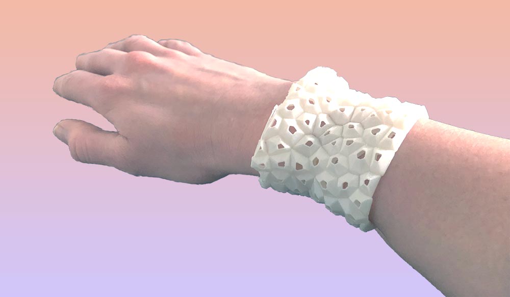
The resulting bracelet!

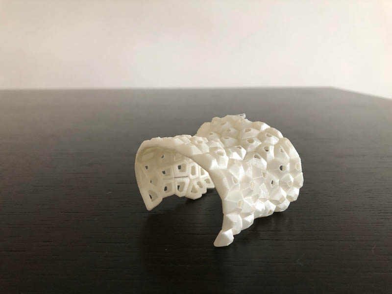
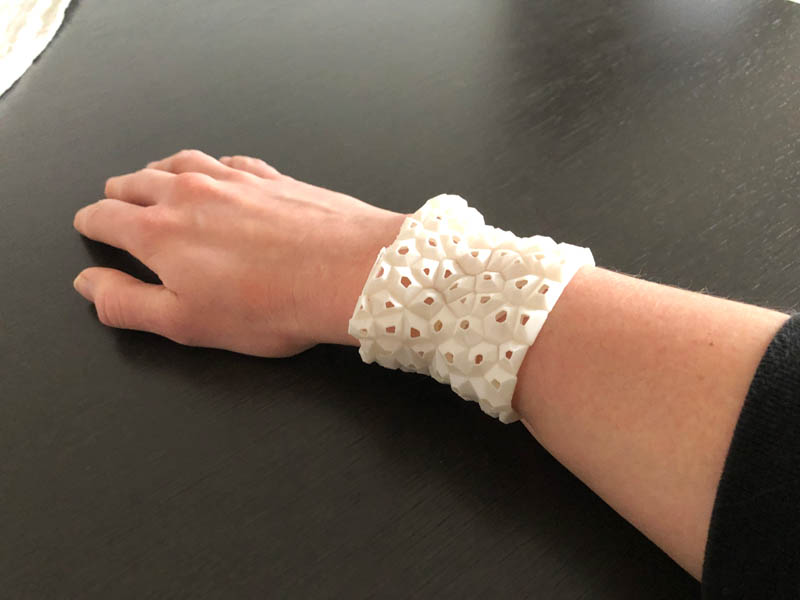
And the hero shot of me wearing it.

Back to top

3D scanning

The second element of this week is 3D scanning. Our task is to 3D scan an object, try to prepare it for printing (and optionally print it). The learning outcome is to demonstrate how scanning technology can be used to digitize object(s). My objective for this week is to scan body parts. The reason is two-fold: for the wristband of this week’s assignment and in preparation of my final project for which I’m designing head- and torso pieces. For this assignment I tested several 3D scanning hardware and software applications. This helps in determining the status of the technology and in selecting the ones that perform best for this purpose.

The tested hardware includes:

• 3D Sense
• Occipital Structure Sensor Mark II
• iPhone 8+ camera

And the following software applications are tested:

• 3DsizeME
• Skanekt
• Qlone app

In the sections below, the results of scanning tests with all these tools are shown. After the tests, a comparison and overall review is given.

Back to top

3D Sense

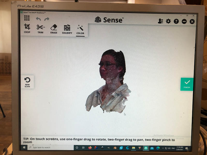
First we start with 3D Sense. At Waag, there is a hand scanner from 3D Sense, with accompanying software. This is what the user interface looks like.

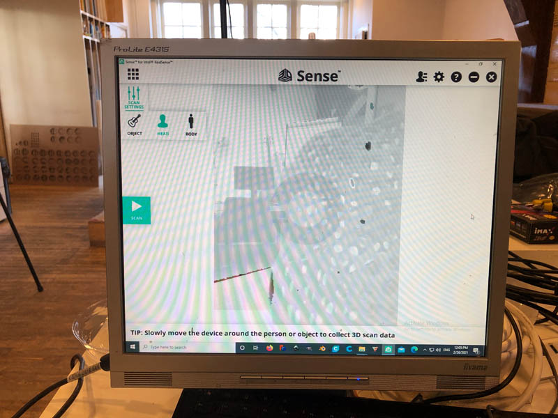
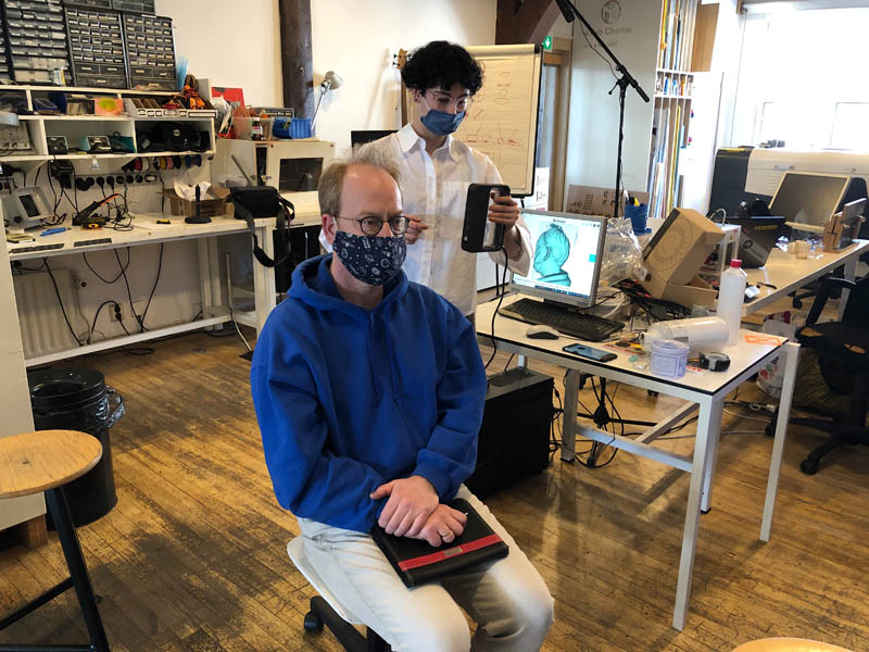
And the sensor in action, while Michelle is scanning Erwin’s head. You have to sit very still in order for the scanner not to lose track on you. When it’s lost, you have to move the scanner back to a previous position. However, this exact position is often hard to find. That results in having to redo the scan.

After that, my head was scanned. This is the front side. A part of my head and chin is missing.

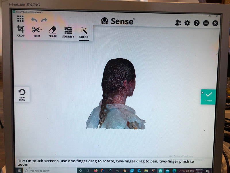
And back side. As you can see, I have two ears.

After this, my head was scanned a second time. Again, the results were disappointing. I exported the .obj file and imported this in Rhino. I will not show you the results, because it’s a really ugly mesh!

Here is a summary of some specs and my experience:

Scanning time	Slow, 5-10 minutes
Scanning precision	Medium
Scanning experience	Easily loses track, requires a lot of focus
Hardware	Handheld 3D scanner connected to PC with cable
Software	Desktop application included with scanner
User interface	Simple and intuitive, very little features
File sharing	Exporting files works well on PC
Costs	+/- €500

The advantages and disadvantages are:

Advantages:

• User interface is easy for beginners
• Exporting files works well

Disadvantages:

• Does not scan uneven textures like hair well
• Slow scanning process, quickly loses track
• Large scanning device, must be connected to PC
• Not compatible with Mac OS

Note: Sense 1 and Sense 2 scanners have been discontinued and are not available for sale anymore.

Back to top

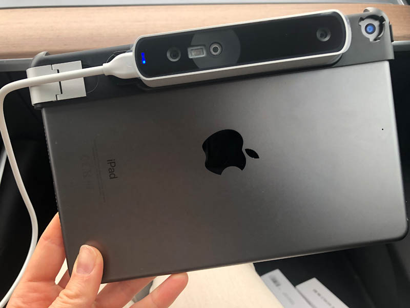
Occipital Structure Sensor Mark II

The following tests are done with the Occipital Structure Sensor Mark II adapter on an iPad Mini.

With this scanner, I tested two Software applications: Skanect and 3DsizeME.

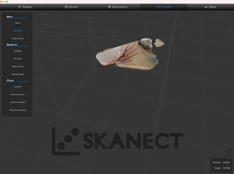
Skanekt

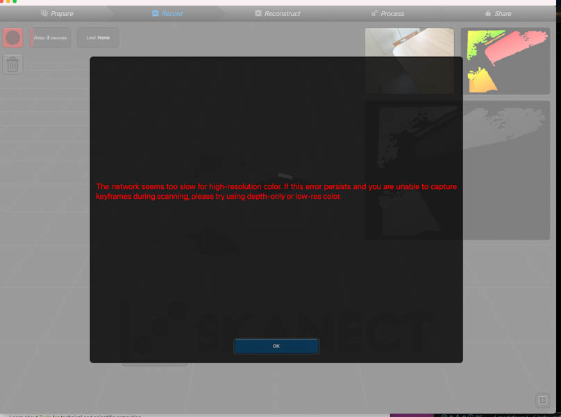
First we start with Skanect, because this is the desktop application developed by the makers of the Occipital sensor. Its user interface has five steps: Prepare, Record, Reconstruct, Process and Share. Your scanner needs to be in close proximity of the PC in order to communicate and to see what you’re scanning.

In the Prepare tab, I set the resolution to High and selected High-Resolution Color. I also selected a box frame of 15x15 cm, fitting the size of my hand and arm. This is what happened.

I changed the color to Low-Res Color and here you see the first attempt to scan my hand. Yes, everything was scanned, except for my hand.

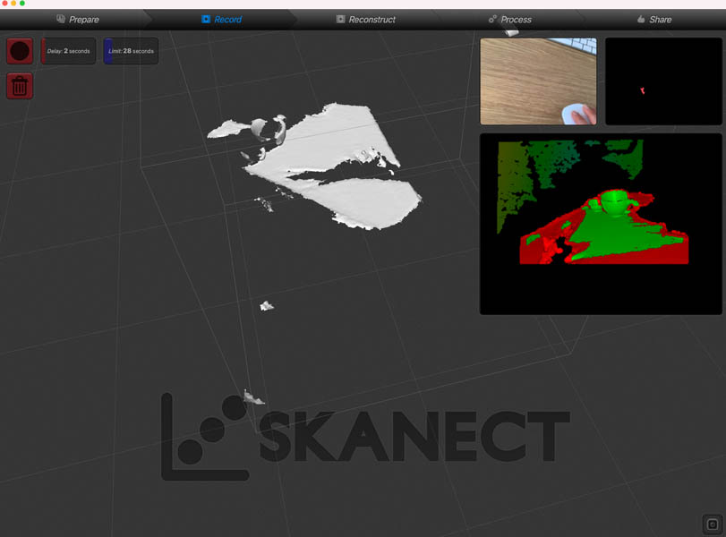
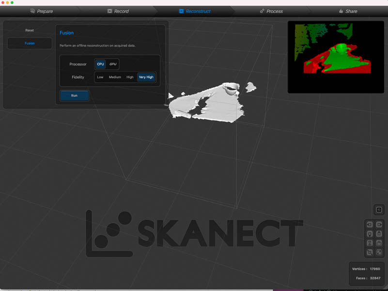
Then in the Reconstruct tab, you can change the settings. I set the Fidelity to Very High in the hope that something good will come out.

Next, the Process tab offers a bit more functions. I made the mesh Watertight and experimented with other settings, like color.

With the Share tab I exported the .obj file and imported this in Rhino to actually see a bit better what was created. First response: “what the heck…”

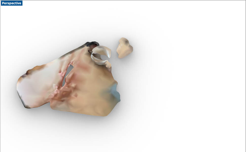
We then repeated this process and made a new scan on a windows computer. Unfortunately this gave comparable poor results.

Here is a summary of some specs and my experience:

Scanning time	Medium, 5 minutes
Scanning precision	Very low
Scanning experience	Horrible
Hardware	Scanning device and bracket for iPads and iPhones
Software	Desktop application sold separately with scanner
User interface	Horrible and old-fashioned, doesn’t work properly
File sharing	Exporting .obj files works well on PC
Costs	Occipital sensor +/- €550, iPad mini bracket +/- €80, software +/- €200

The advantages and disadvantages are:

Advantages:

• None

Disadvantages:

• Expensive
• Doesn’t scan what you want
• Terrible user interface
• On a Mac OS lots of issues kept reocurring, such as non-compatibility with graphics card
• You have to be connected to a PC to scan, and look at your desktop screen to scan instead of the iPad. This is counterintuitive.
• Sensor and iPad out of battery within 5-6 scans, iPad becomes really hot

So all in all, Skanect was a bad experience.

Back to top

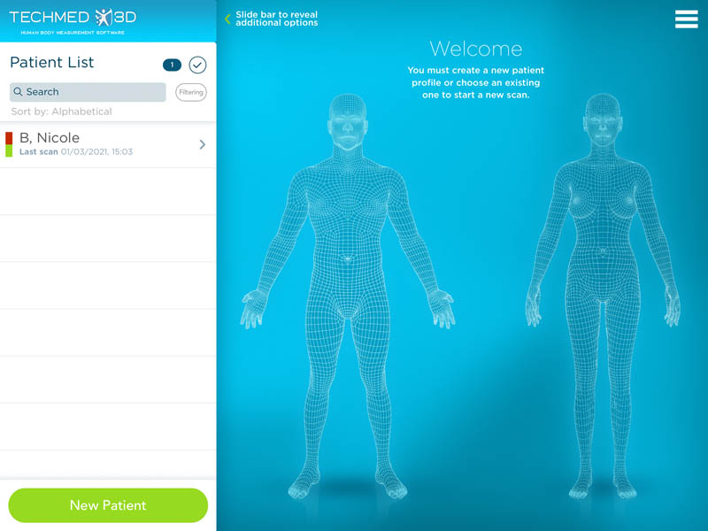
3DsizeME

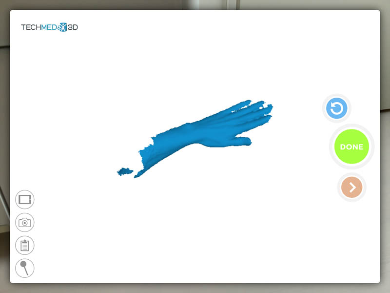
The second application I’m testing with the Occipital Structure Sensor Mark II is 3DsizeME from Techmed3D. This is professional human body measurement software for medical applications. I came across this app at the orthophedic shoemaker factory, where they also produce custom-made ice skates. Let’s hope that this software tool is better! The user interface already is a major improvement. To make a scan, you have to create a new “patient”. Then select the body part you want to scan.

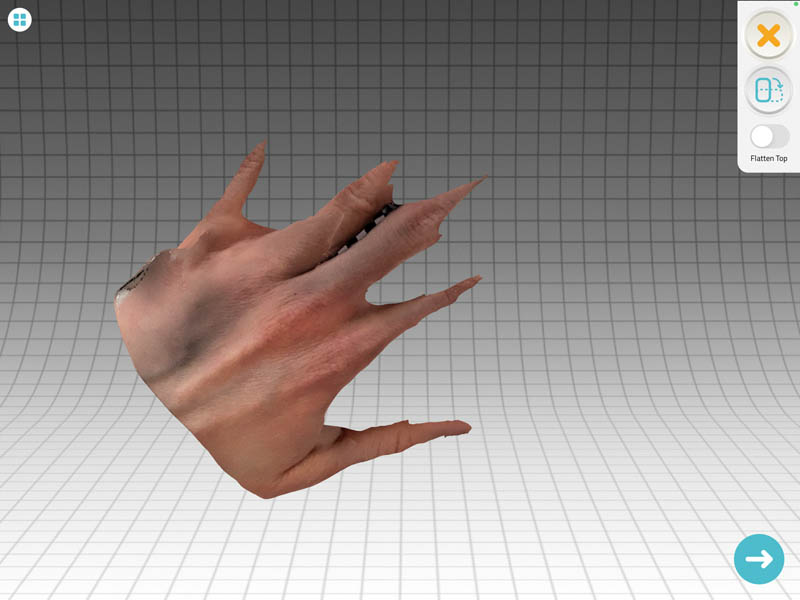
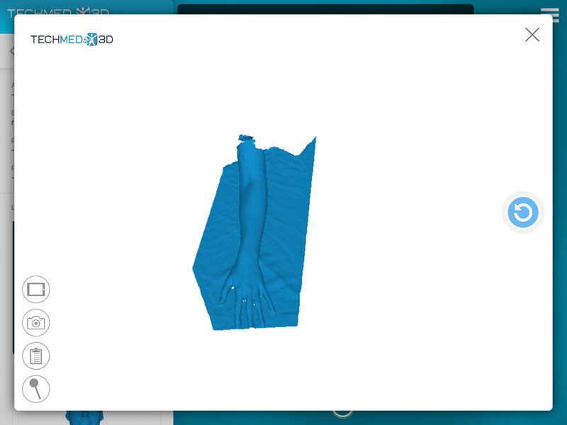
This is the first scan of my hand. Not bad at all! It shows a lot of detail and distinguishes the target object from the background.

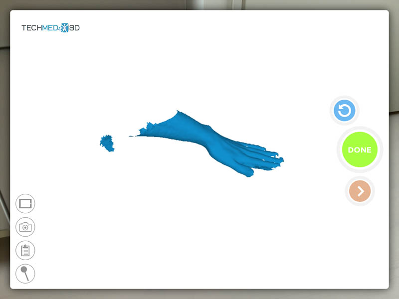
Another scan also gave a nice result, this time the background was included. After scanning, you can cut out a frame. There are not a lot of other post-processing options. But that’s fine because the quality of the scan is good.

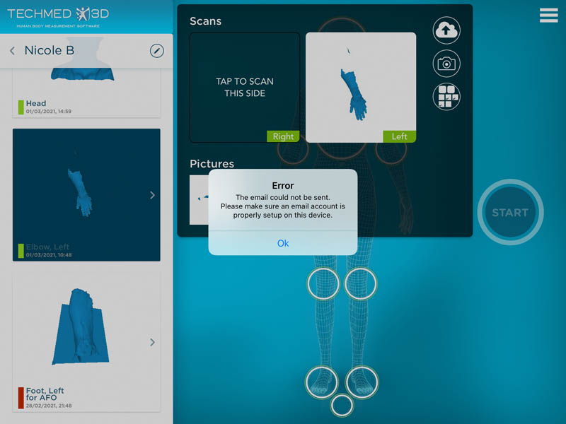
Then, it’s time for exporting! And this error really sucks… I tried all possible ways but 3DsizeME was not able to share the file.

Here is a summary of some specs and my experience:

Scanning time	Fast
Scanning precision	Good
Scanning experience	Medium, sometimes the box jumps, which is annoying
Hardware	Scanning device and bracket for iPads and iPhones
Software	Mobile application freely available in app store
User interface	Beautiful, however you can only select a few body parts with the circles (not your hands for example)
File sharing	Exporting files doesn’t work
Costs	Occipital sensor +/- €550, iPad mini bracket +/- €80, software free

The advantages and disadvantages are:

Advantages:

• Good quality of scan
• Beautiful and good-working user interface
• You can scan anywhere, without the need for cables and PCs
• If you’re a doctor, this app offers a good file management system for information about your patiens

Disadvantages:

• Doesn’t export files!!
• Scanning is bit of a black-box: very few options for changing settings

Conclusion: compared to the previous tools, I’m impressed by the quality of the scans. However, it’s really disappointing that the files can’t be shared.

Back to top

Qlone app

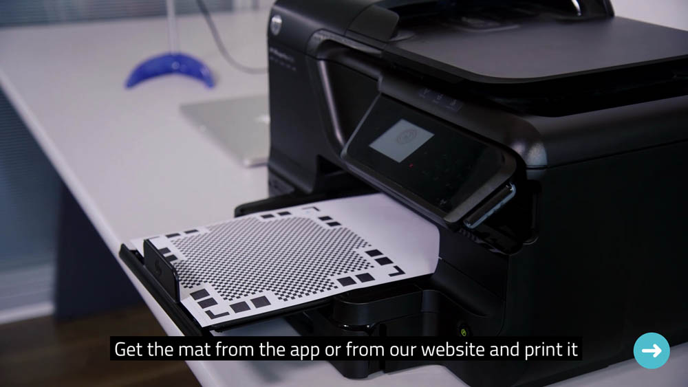
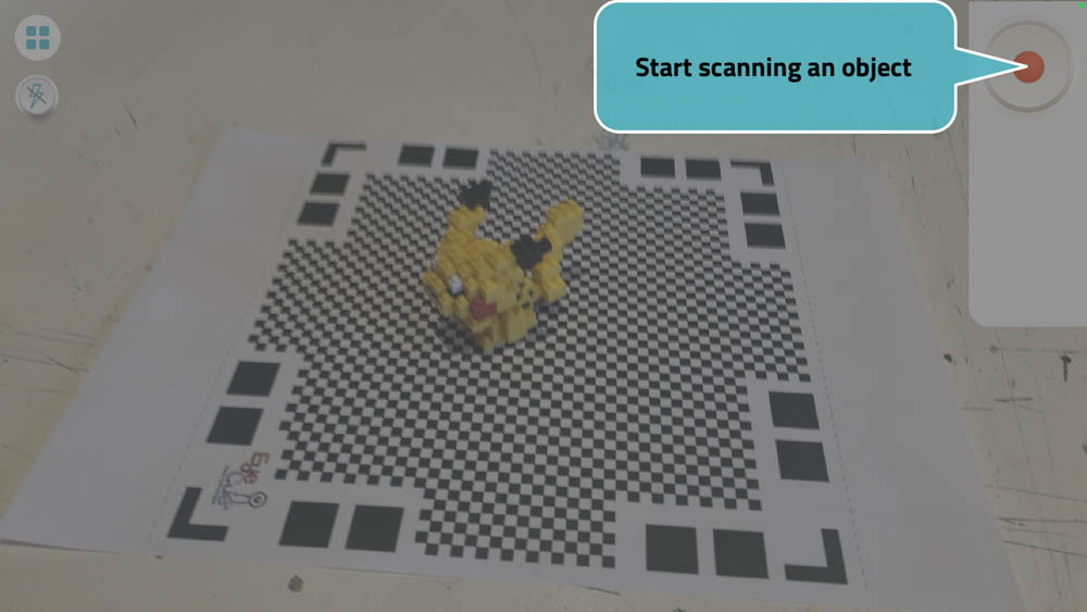
The Qlone mobile application can be downloaded on phones and iPads and doesn’t require additional hardware. When you open the app, a clear step-by-step guide shows what you need to do in preparation of the scan. First, you print a Augmented Reality (AR) mat with a regular printer. This is required to recognize the object.

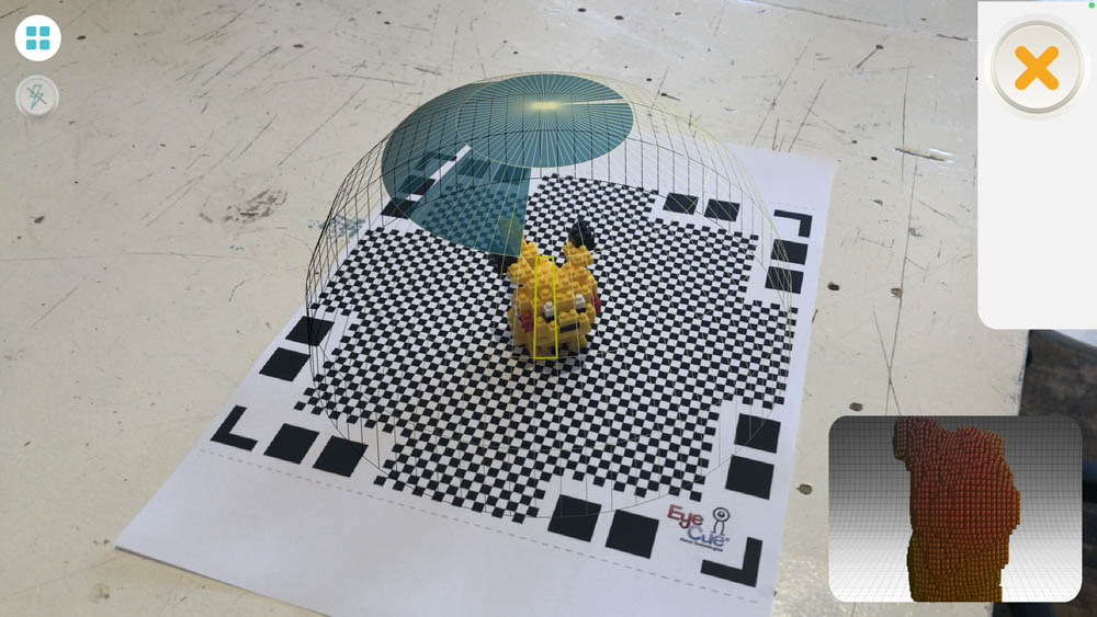
Next, you place the object on the AR mat.

With your phone, follow the AR sphere until all sections are blue.

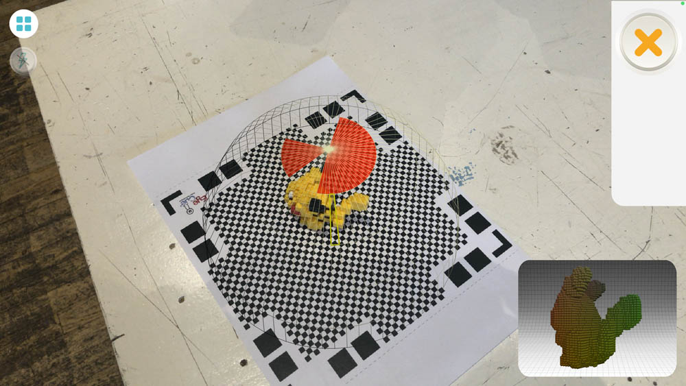
If you lose track the sphere will become red. Navigate back to a previous section to continue scanning.

When you complete the sphere, you can proceed to processing.

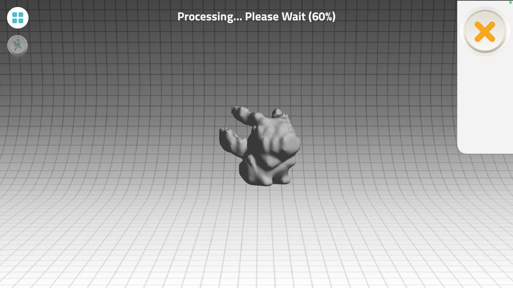
After processing the result is shown. This is not bad! You can rotate the object and export as .gif, .mp4 or .jpg for free. If you want to export to .obj, .stl and other file formats or platforms like SketchFab, you have to upgrade to premium.

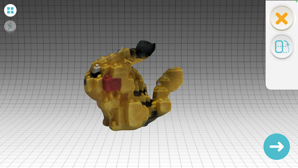
Then the ultimate test, a scan of my hand. I tried to do this twice and unfortunately it doesn’t yield a successful result..

Here is a summary of some specs and my experience:

Scanning time	Medium, filling all segments can take longer than you want
Scanning precision	Medium-Sufficient
Scanning experience	Good for small objects
Hardware	No hardware needed, only a phone and printed AR mat
Software	Mobile application freely available in app store
User interface	Nicely done, clear instructions
File sharing	Exporting files only with premium
Costs	Free app, premium upgrade €22 one-time charge

The advantages and disadvantages are:

Advantages:

• Cheap, if you have a phone
• Medium to good quality of scan
• Nice and good-working user interface
• You can scan anywhere, without the need for hardware, cables and PCs, if you printed the AR mat
• Files can be shared in a variety of file outputs and platforms, great integration

Disadvantages:

• App works better on iPhone than Android
• You can only scan small objects if you don’t have access to a large plotter for printing a huge AR mat
• The app has trouble recognizing the skin

Conclusion: it is impressive that this mobile app can generate better scans than a €600+ hardware-software combination. But still, the technology is not able to recognize skin properly, or to create a precise copy of a lego object.

Back to top

Comparison between 3D scanning hardware and softwares

My overall conclusion of this assignment is that 3D scanning technology is not quite there yet. The impression is that this limitation seems to be more about the software than the hardware. For example, Occipital’s Structure Sensor Mark II addition to an iPad performs significantly better in the 3DsizeME app compared to Skanect software. Also, in general the mobile applications seem to bypass the hardware products at a rapid pace. 3DSense’s Sense 1 and Sense 2 scanners have been discontinued and are not available for sale anymore. It is also harder to find the Structure sensor in the Netherlands. The Augmented Reality feature of the Qlone app is a smart way to improve scanning quality, reduce costs and create more flexibility. I believe this digitalization trend will continue, so that in a few years we only need a phone. In fact, it’s already here with the new LiDAR scanner on an iPhone 12. I’m curious to the performance of this scanner and if this will live up to its premise.

3D scanning assignment

To prepare for my final project I gave myself an extra challenge to design a workflow from 3D scanning to parametric design and 3D printing. This was for the bracelet design, in the section on 3D printing above. Unfortunately, due to the poor image quality or file output of all scanners I was not able to get a good scan of my wrist. Thus, the plan to scan my wrist, design the bracelet around it in Rhino and Grasshopper, and then 3D print it didn’t work out.

In a larger context, beyond this assignment, I hoped to scan mechanical parts of existing objects, and design additions around it. Complicated surfaces like skins are hard to scan. But also square-like objects turned out to be difficult for 3D scanners, and are smoothened out as we saw in the Qlone app example. So all in all, I would not trust this technology for creating technical parts. Old-school measuring still works best.

Back to top

Downloads

• Bracelet design Grasshopper file (.gh)
• Bracelet design Rhino .3dm file (link to Google drive)
• Bracelet .stl file (link to Google drive)

Some notes from lecture Neil

On 3D printing and 3D scanning.

3D printing

• 3D printing can give off nasty fumes. Only PLA is safe for tabletop printers in the office and at home.
• Overview of 3D printing materials by Prusa
• Arc Welder is an Octoprint plugin for smoother 3D prints. It creates gcode that substantially compresses the file and may reduce stuttering.
• Clearance - design with space in between the objects. example.
• This week, check in CAD files not the STL files as they might be too big.
• It’s very easy to write STL file in code. You don’t need CAD program if you’re good at programming.
• Nonplanar.xyz
• ‘gcode is way past its due date’ - Neil (24 february 2021)
• Design rules for printer:
  • Angle - can be done without support
  • Bridging - can also be done without support!
  • These two techniques combined are very powerful.
• Questions to ask:
  • How far can you bridge?
  • What are the tolerances?
  • What can you do without support?
• Circular design:
  • Filastruder
  • Precious Plastic
• Two objectives of this week:
  1. Avoid thin features where the printer will fail.
  2. Learn to design without needing support.

3D Scanning

• Openscan
• Most state of the art: light
• Specscanning - spherical harmonic illumination. Measures the light transmission field and creates a 3D reconstruction.

Back to top