Assignment Requirements
Individual assignment
- Read, sign (add your name to) the student agreement and commit it to your repo
- Work through a git tutorial
- Build a personal website in the class archive describing yourself and your final project. Refer to the lecture material for examples
- Upload parts 1 and 2, to the class archive
Progress Status
Group page link + notes added.
Missing final photos and conclusions.
Upload .zip with source files.
1) Introduction
My interest in 2D and 3D design software began at the early stages of my academic path, first through interior design studies and later during my architecture education. Throughout these years, working on different types of projects has allowed me to explore a wide range of digital tools, each one responding to specific design needs, from technical documentation to conceptual exploration and fabrication. This process has not been linear. Instead, it has been shaped by experimentation, professional practice, and exposure to different design methodologies, which helped me understand how each software operates within a broader design ecosystem.
2) 2D Software Experience
At a 2D level, I have worked mainly with: AutoCAD, as my primary tool for technical drawings, plans, sections, and construction documentation. Adobe Illustrator, for vector-based design, diagrams, graphical layouts, and technical illustrations. CorelDRAW, which I explored earlier in my academic formation, mainly for vector graphics and layout work. Adobe Photoshop, used for raster-based work such as image editing, collages, visual studies, and graphic compositions. These tools allowed me to clearly understand the differences between raster and vector workflows, and how each one plays a different role in architectural representation and communication.
Examples of raster work in Photoshop, vector drawings in Illustrator, and 2D plans in AutoCAD
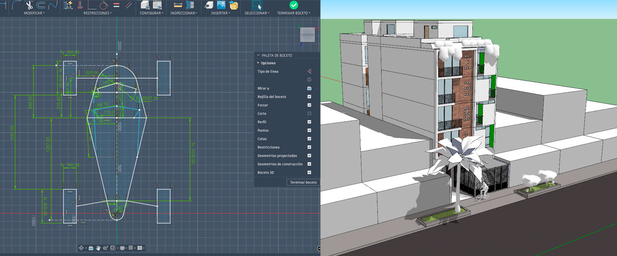
3) 3D Software Experience
My strongest experience is in 3D modeling, due to my background in architecture and the variety of tools I have used over time. These include: SketchUp, mainly for fast volumetric studies and conceptual modeling. Fusion 360, especially for parametric modeling, product design, and fabrication-oriented workflows. Revit, for BIM-based architectural modeling and coordinated documentation. Rhinoceros + Grasshopper, which has become one of my most important tools for parametric design, geometric exploration, and system-based thinking. Blender, used for animation, simulation, and experimental geometry. 3ds Max, explored for rendering and advanced visualization. D5 Render, for real-time rendering and architectural visualization. Through these tools, I have worked on modeling, rendering, animation, and simulation, allowing me to approach design from both a technical and experimental perspective.
Selected images of 3D models, renders, animations, and simulations produced with these tools
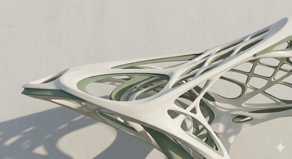
4) Final Project
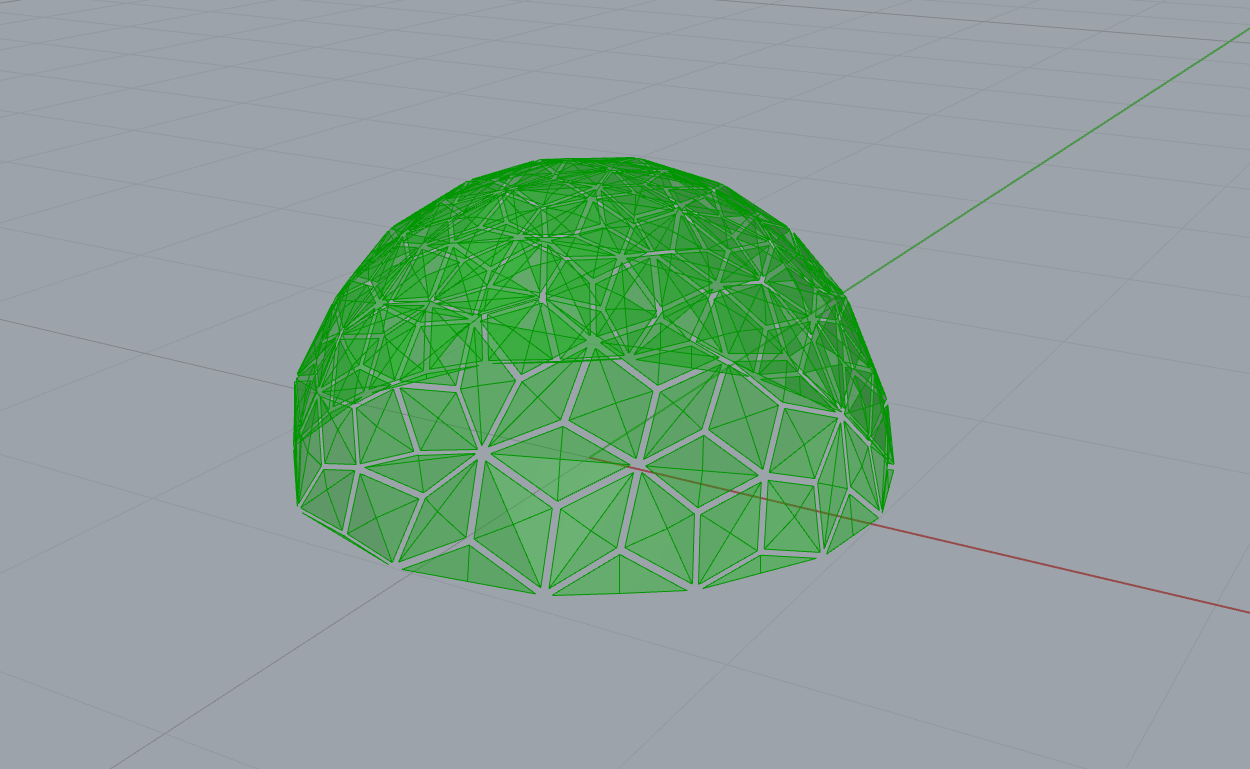
This project is part of an ongoing architectural research focused on adaptive and regenerative construction systems. Rather than designing a final object, the goal of this stage was to explore how a parametric geometric system could translate territorial, material, and environmental variables into a controllable architectural structure. For this first cycle, the work focuses on developing a parametric dome-based system composed of triangular modules, which later will be capable of reacting to environmental conditions such as solar exposure through kinetic behavior.
The image above shows the initial parametric dome geometry generated in Grasshopper. This structure represents the base system before introducing kinetic behavior or environmental interaction.
5) Process – First Attempt: Regenerative Matrix as Parametric Inputs
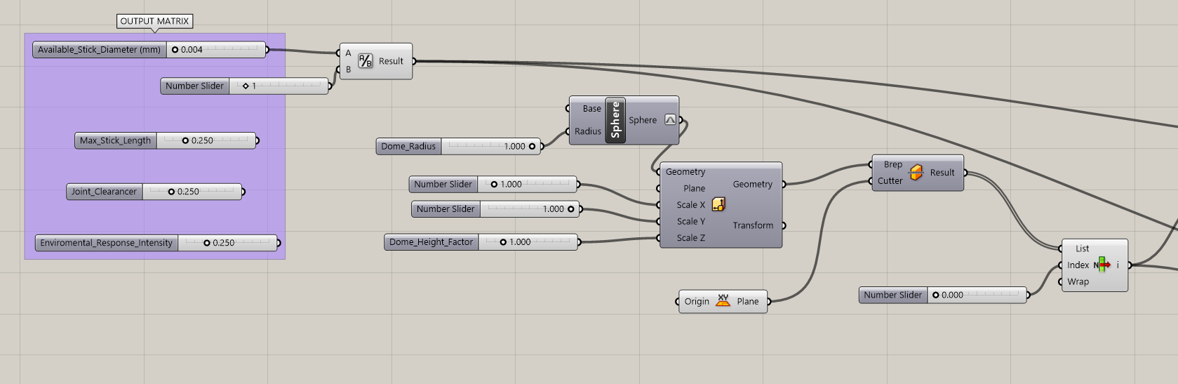
Before generating any geometry, I created an Output Matrix that translates concepts from regenerative architecture into parametric values. These parameters are not purely geometric; they represent territorial and material constraints that could later be tied to real construction conditions.
Step 0:Output Matrix Parameters
- Available_Stick_Diameter (mm) Represents the diameter of wooden sticks or bamboo elements available in the territory.
- Max_Stick_Length (m) Defines the maximum length of structural elements that can be harvested or transported.
- Joint_Clearance (mm) Introduces fabrication tolerance and construction gaps between elements.
- Environmental_Response_Intensity (0–1) Controls how reactive the system is to environmental stimuli (this parameter will later influence kinetic behavior).
Step 1: Sphere Creation
- A Dome_Radius slider was connected to the Radius input of the Sphere.
- This allowed full control over the overall scale of the structure.
Step 2: Proportional Control Using Scale NU
- Scale X and Scale Y were kept at 1.0
- Scale Z was controlled using a Dome_Height_Factor slider
Step 3: Creating a Half Dome
- The geometry was connected to a Brep | Plane Split component
- A World XY Plane was used as the cutting plane
- The resulting Breps were passed into a List Item component
- By selecting the appropriate index, only the upper half of the sphere was kept
Step 0/1/2/3
Step 4: Mesh Conversione
- The selected half-dome Brep was converted into a mesh using Mesh Brep.
- This step was necessary to allow further operations such as remeshing, edge extraction, and panelization.
Step 5: TriRemesh for Uniform Triangles
- The Module_Size slider was connected to the Target Edge Length input
- This parameter controls: Density of the structure / Size of each triangular module / Overall visual and structural resolution
Step 6: Extracting Structural Edges
- From the remeshed geometry, I extracted the edges using Mesh Edges.
- These edges represent the structural framework of the system.
Step 4/5/6
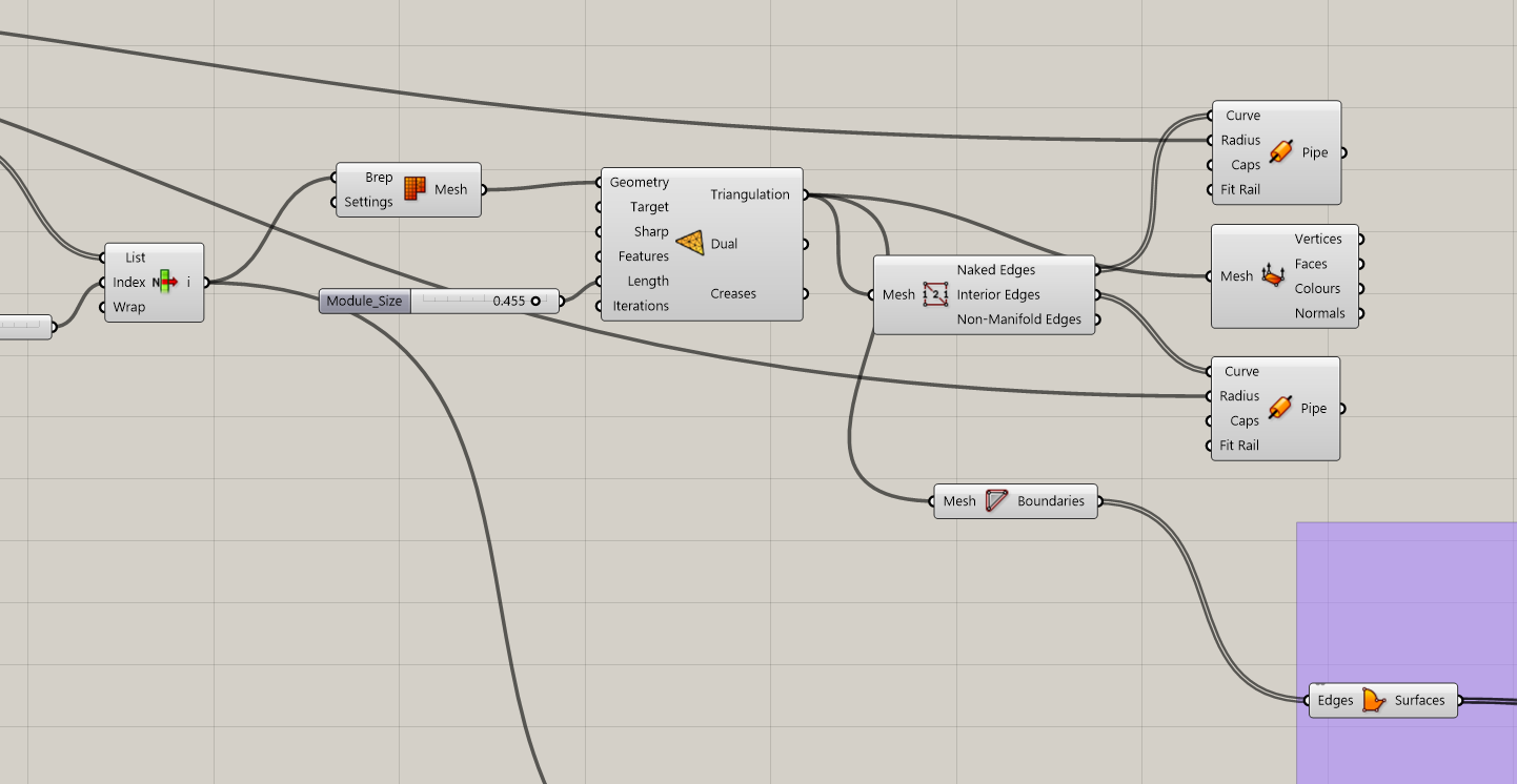
Step 7: Face Boundaries to Surfaces
- The remeshed geometry was connected to Face Boundaries
- The B (Boundaries) output was then connected to Boundary Surface
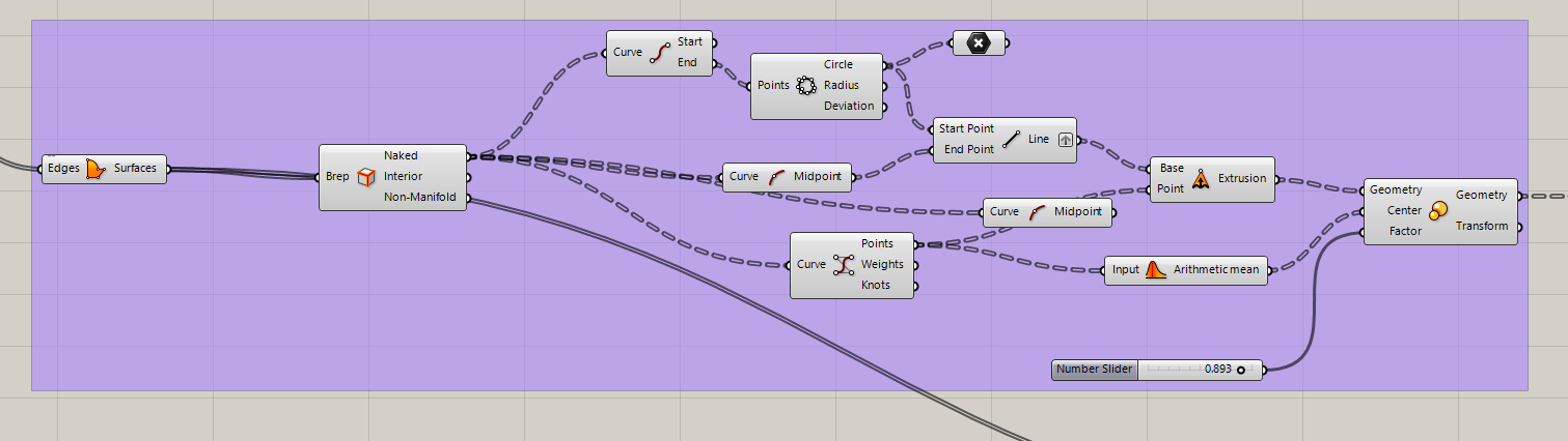
Step 8:Early Kinetic Exploration (First Attempt)
- With triangular surfaces generated, I began exploring how each panel could act as an independent unit. Midpoints of edges were evaluated
- Simple vector directions were tested
- Early transformations were applied to simulate opening behavior
- This stage involved several errors and broken definitions, which were part of understanding: Data trees
- Matching geometry to motion
- Maintaining coherence between panels
Step 7/8
Step 7/8
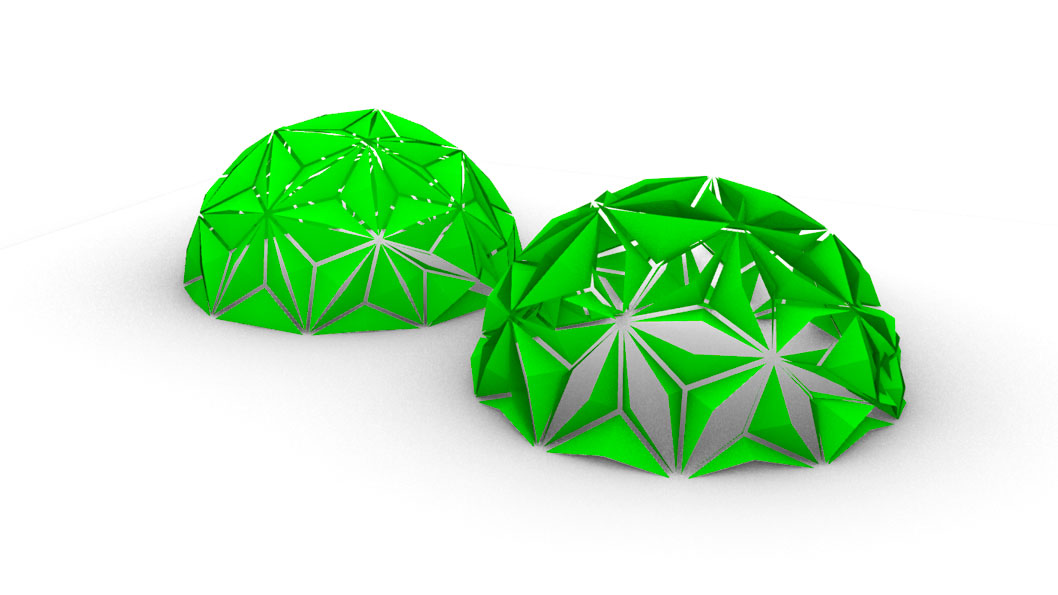
Semi-dome geometry after triangulation, showing a relatively uniform distribution of triangular panels. This configuration was used to evaluate structural density, module size, and the feasibility of treating each triangle as an independent kinetic unit.
First Attempt
Reflection on This Stage
- This stage focused on geometry, structure, and parametric logic rather than producing a final solution.
- Several iterations were required to understand how mesh topology affects panel behavior and data flow.
- Clean and uniform triangulation proved to be critical for any future kinetic movement.
- Many errors and broken definitions helped clarify how data trees operate in complex systems.
- Working step by step allowed the system to remain flexible and adaptable instead of over-defined.
- At this point, the project establishes a solid geometric and structural foundation for future environmental interaction.
Errors & Fixes
- Initially, the dome geometry was generated using a circular profile that was later cut in half to obtain a semi-dome.
- However, this approach consistently produced a central node at the top of the dome, where multiple vertices converged into a single point.
- This geometric condition is inherent to how circular and spherical geometries are parameterized in Rhino, especially when working with revolutions and trimmed surfaces.
- To explore an alternative solution, a second method was tested by generating a dome through an arc profile and using a surface of revolution.
- This revolved surface was then connected to the LunchBox Triangle Panels Beam component to generate triangular panels.
- Although this method successfully produced a dome-like surface, the triangulation resulted in overlapping panels and a strong concentration of vertices at the apex.
- The main issue was that the Triangle Panels component requires a well-distributed surface parameterization.
- Due to the rotational nature of the geometry, all surface isocurves collapsed at the top point, forcing all triangular panels to converge into a single central node.
- This prevented the generation of uniformly sized triangular modules, which was a key objective for developing independent kinetic panels.
First Error
Geometric Issue: Central Node Concentration in Dome Generation
This exploration highlighted an important limitation when using revolution-based geometries for panelization. Understanding this behavior was essential in deciding to shift towards mesh-based remeshing workflows, where vertex distribution can be controlled more precisely and without singularities.
6) Process – Second Attempt: Parametric Inputs
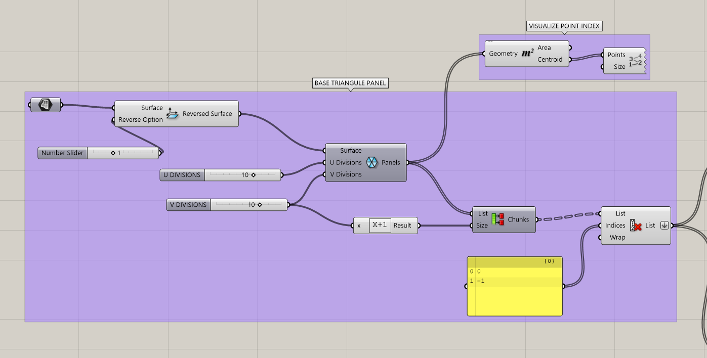
Base Triangle Panel System
After several attempts to generate a uniform triangulated dome surface, I decided to step back and rethink the problem from a more controlled and modular perspective. Instead of forcing a dome geometry from the beginning, I focused on developing a base triangular panel logic that could later be applied to any surface.
This approach allows the system to remain flexible and scalable, while avoiding common geometric issues such as vertex concentration, central nodes, or uneven triangulation.
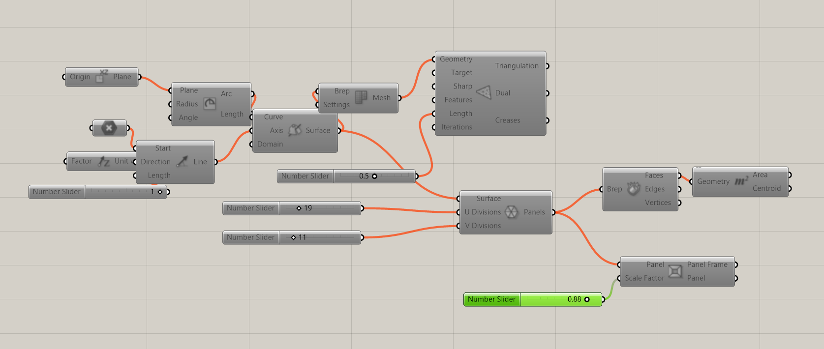
The base input of this system is a simple surface referenced directly from Rhino. In this case, a rectangular surface was used, but the logic is designed to work with any planar or curved surface in future iterations.
- The surface is referenced into Grasshopper as the main geometric input
- This allows the triangular system to adapt to different architectural elements
- The logic is no longer tied exclusively to domes or rotational geometries
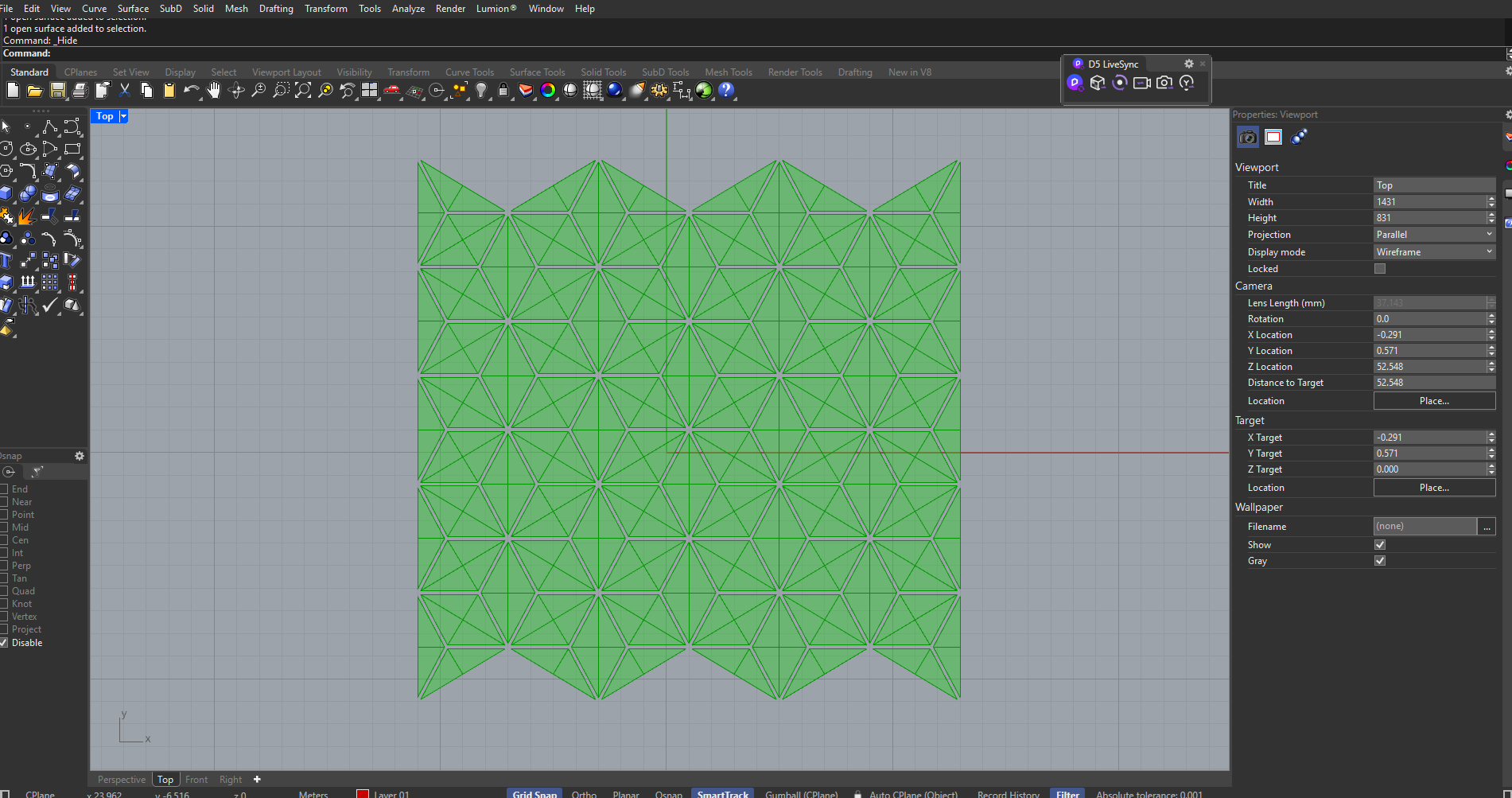
Triangular Panels Generation
The referenced surface is then connected to the LunchBox plugin component Triangle Panels B, which subdivides the surface into a triangular grid. The U and V division sliders control the density and scale of the panels.
- U Divisions define the horizontal subdivision density
- V Divisions define the vertical subdivision density
- This provides full control over panel resolution and module size
Cleaning the Panel List
One important issue with panel-based subdivision systems is that the boundary panels are often incomplete or irregular. These partial triangles are not useful for fabrication or for kinetic behavior.
To solve this, the resulting panel list is processed using list management components:
- The panel list is divided into chunks
- Specific indices are removed using list item selection
- Only complete triangular panels are kept
This step ensures that the final output is a clean and consistent set of triangular modules, suitable for both digital simulation and future physical fabrication.
Resulting System Logic
By separating the panel logic from the dome geometry, this system becomes a reusable architectural tool rather than a fixed form.
- The same logic can be applied to walls, roofs, facades, or freeform surfaces
- Each triangle can later act as an independent kinetic unit
- This prepares the system for environmental responsiveness and actuation
This base triangular panel system becomes the foundation for the next stages of the project, where each panel will be assigned orientation logic, hinge behavior, and environmental inputs such as solar exposure.
Commands - Results
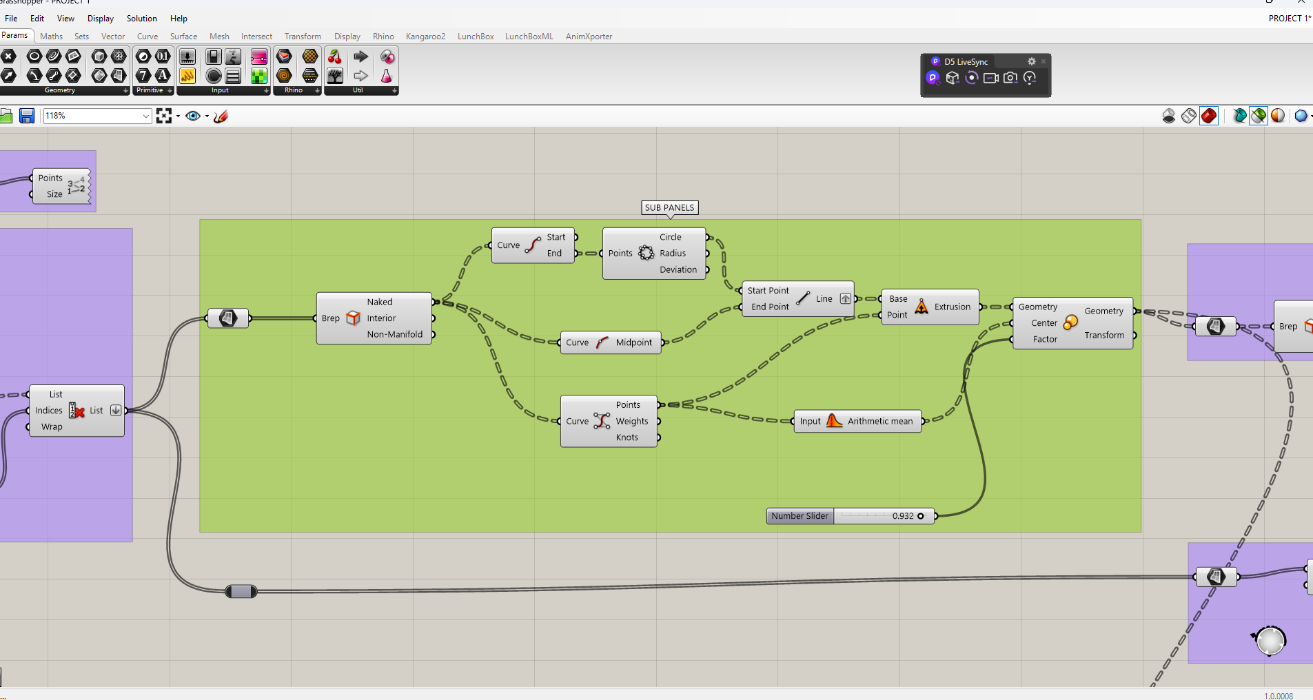
Sub-Panels Generation and Spacing Control
After defining the main triangular panel system, the next step was to explore how each panel could be subdivided into smaller internal elements while maintaining geometric coherence and control.
- Starting from the cleaned list of triangular panels, the edges of each panel were extracted to understand their internal geometric structure.
- Using the edge data, midpoint calculations were performed to identify secondary reference points inside each triangle.
- These midpoints allowed the generation of internal sub-panels that remain proportional to the original triangular geometry.
- An arithmetic mean operation was applied to define a central reference point for each panel, ensuring consistent scaling behavior.
- A Scale transformation was then applied to each sub-panel using its own center as a pivot.
- The scale factor acts as a spacing controller, defining the gap between panels and allowing the system to open or densify parametrically.
This approach transforms each triangular unit into a controlled kinetic-ready module, where spacing, porosity, and visual permeability can be adjusted without breaking the overall system logic.
Commands - Results
Kinematic Logic: Length and Area Preserved Motion
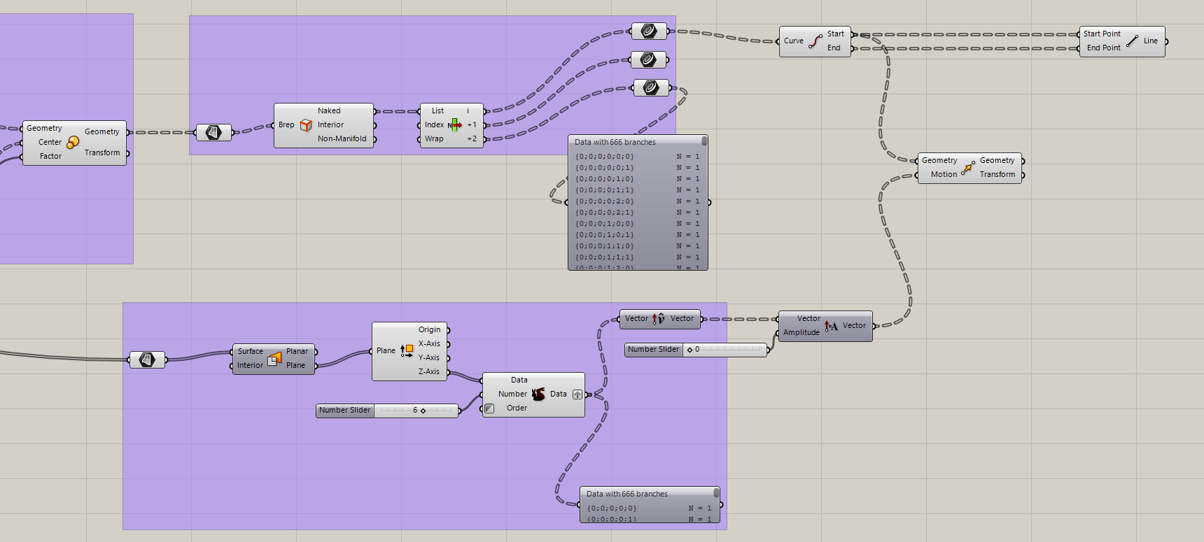
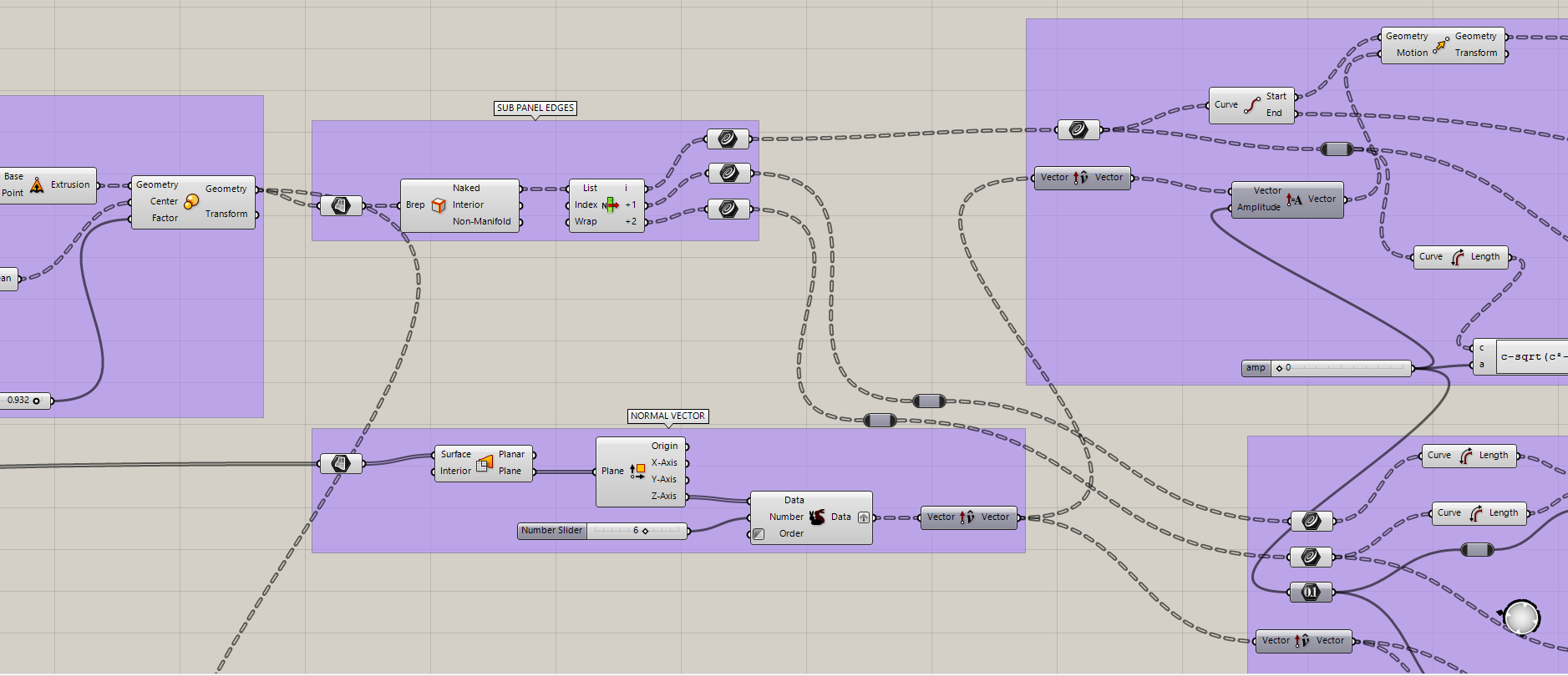
This stage represents one of the most complex but also most important moments of the project. After defining the internal spacing of each sub-panel through scaling, the geometry was reorganized to begin extracting structural and kinematic information from the triangular system.
- Once the scaled sub-panels were defined, their edges were extracted to generate the hinge and motion boundaries of each element.
- From these sub-panel edges, the geometric relationships of each triangle were analyzed, specifically identifying the hypotenuse, adjacent, and opposite sides.
- These values were not used as pure geometry, but as inputs for kinematic control and mathematical consistency.
In parallel, a perpendicular reference direction was required to define controlled motion away from the panel surface.
- Using the original base triangle panels, each surface was evaluated as planar.
- From the construction plane of each panel, a perpendicular (normal) vector was extracted.
- This normal vector represents the direction in which the sub-panel would move away from its base position.
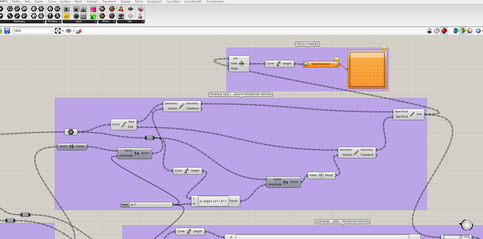
Triangle Side C: Length Preserved Motion
In order to allow controlled movement without changing the physical length of the structural element, a length-preserving motion logic was implemented.
- The hypotenuse of each triangle (side C) was treated as a fixed-length element.
- A motion amplitude factor was introduced using a number slider.
- This amplitude was combined with the perpendicular vector direction to simulate movement normal to the panel.
- To ensure that the hypotenuse length remained constant during motion, a mathematical constraint was applied.
The following equation was used to preserve the length of side C during perpendicular displacement:
c - sqrt(c² - a²)
This expression ensures that even when the element moves outward, its effective length does not change, which is critical for future physical fabrication using rigid members.
Sub-Panel Area Preserved Motion
Beyond preserving edge lengths, it was also important to ensure that the surface area of each sub-panel remained constant during motion.
- Maintaining a constant area allows the use of flat, rigid panels without requiring deformation.
- This constraint is essential for fabrication using planar sheets such as plywood, metal, or composite panels.
- The motion therefore becomes rotational and translational, but not elastic.
Using the geometric relationships between the adjacent, opposite, and hypotenuse sides, a rotation angle was calculated to compensate for movement while preserving area.
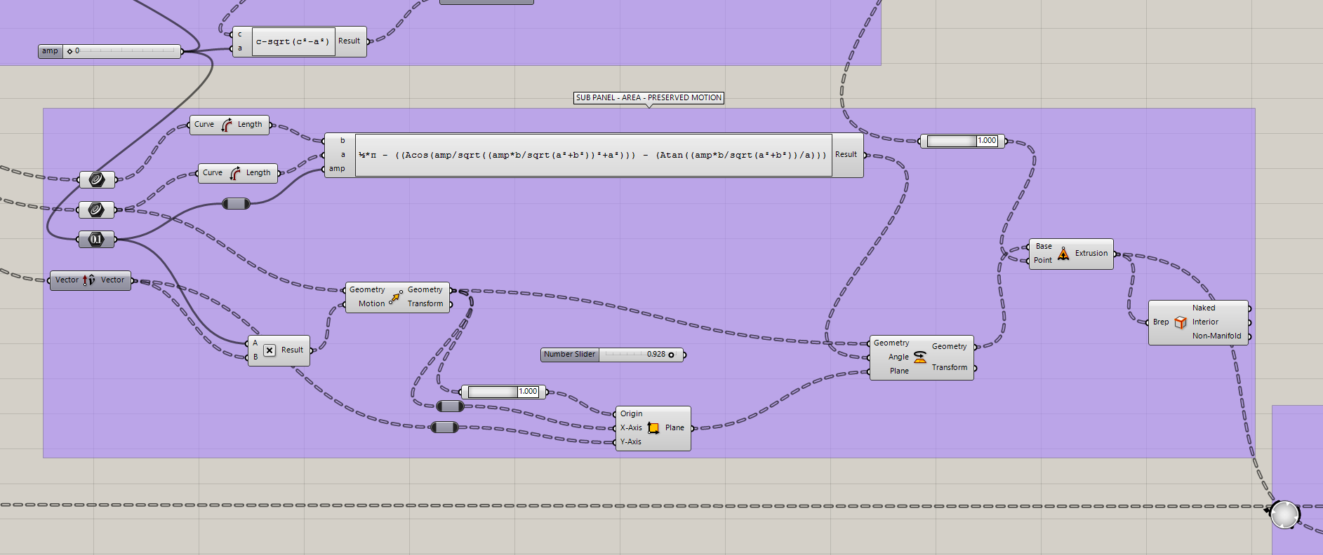
The rotation angle was defined using the following expression:
½·π - ((acos(amp / sqrt((amp·b / sqrt(a² + b²))² + a²)))
       - (atan((amp·b / sqrt(a² + b²)) / a)))
This equation outputs a rotation angle that allows the panel to move while keeping its area constant, effectively locking the panel geometry while allowing kinematic behavior.
By preserving both length and area, the system ensures that all panels can be fabricated as flat elements. This shifts the complexity of the system away from material deformation and into the connector design, which becomes the true site of innovation.
At this point, the kinematic logic is geometrically validated. The next stage will involve applying a transformation matrix to coordinate motion across multiple panels, and later integrating animation and physical actuation strategies.
Sub Panel Edges + Normal Vector
Triangle Side C - Length - Preserved Motion
Sub Panel - Area - Preserved Motion
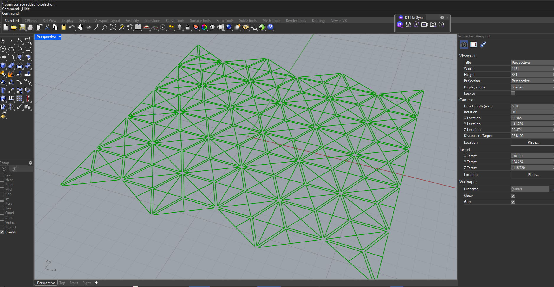
Model: Amplitude 0
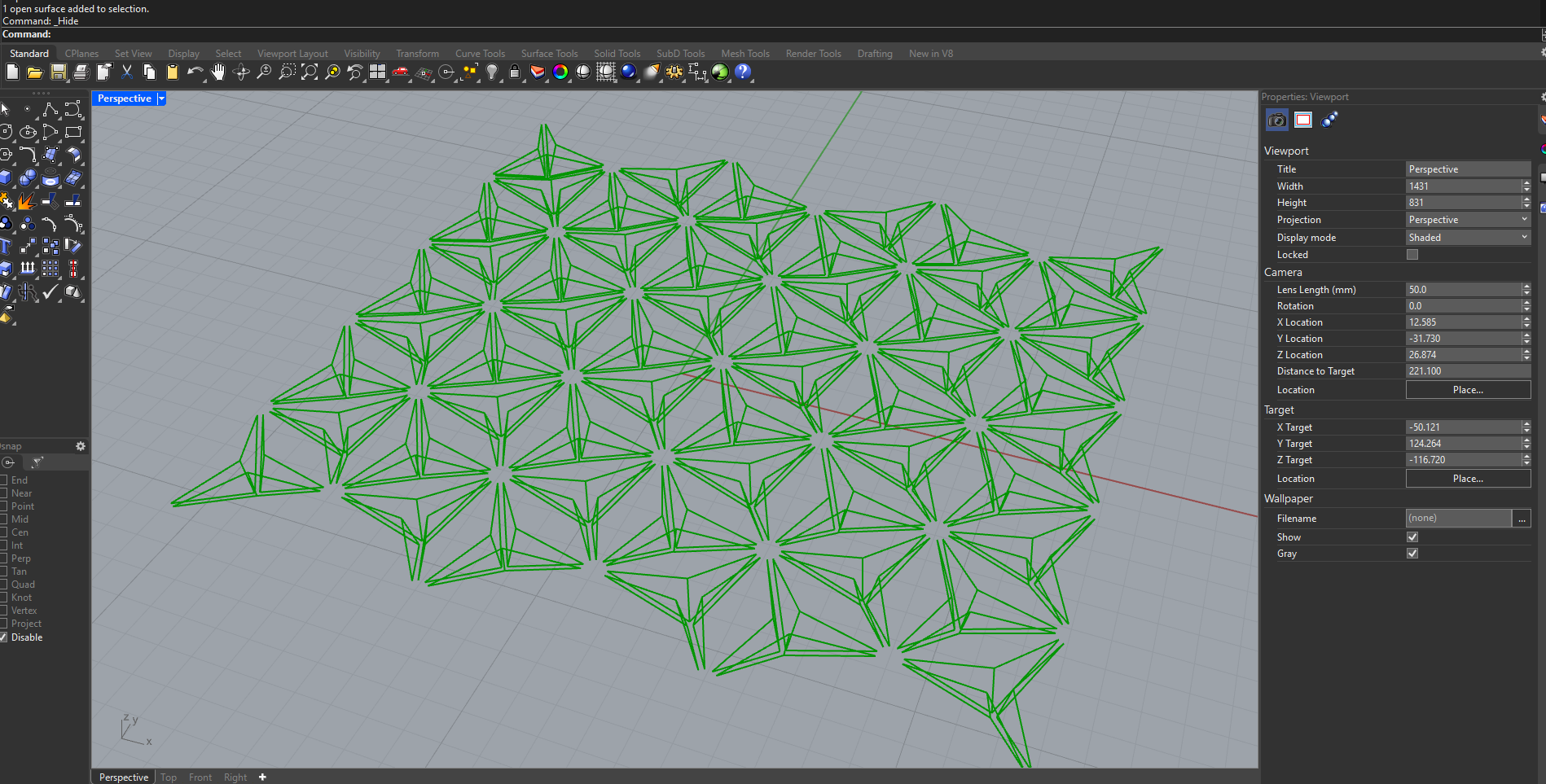
Model: Amplitud 1
Final Geometry Integration – Dome as System Carrier
- For the final stage of this exploration, a dome geometry was introduced as the base carrier for the entire system. In this case, the dome is not treated as a final architectural form, but as a geometric support used to test how the previously developed logic behaves when applied to a curved surface.
- The original base triangle panel input was replaced by a hemispherical dome surface generated directly in Rhino. This surface was then referenced into Grasshopper and used as the new input for the triangular panel system.
- Once linked, all previously defined rules — panel subdivision, subpanel generation, kinematic constraints, and preserved-length and preserved-area motion — were automatically replicated across the entire dome surface.
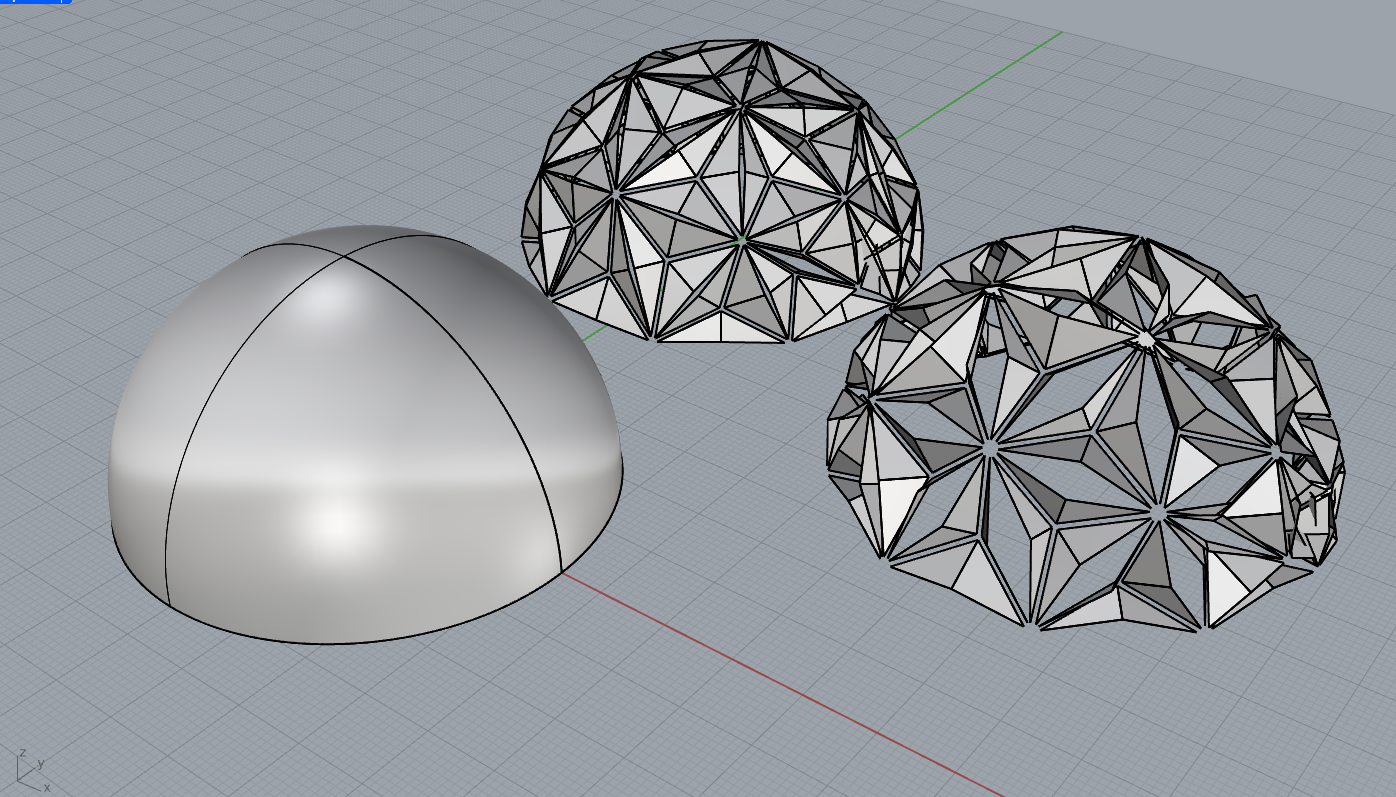
Reading the Geometric States
- On the left, the image shows the original dome as a smooth geometric primitive, representing the neutral and undeveloped state of the system.
- In the center, the same dome is displayed after applying the triangular panel logic. At this stage, the surface is discretized into a dense network of triangular panels, each carrying internal geometric complexity derived from the subpanel system.
- On the right, the amplitude trigger is activated. This parameter controls the magnitude of the kinematic transformation, allowing the panels to open and deform while maintaining their geometric constraints.
System Behavior and Next Steps
- This final test demonstrates that the system is not bound to a single form. The same logic can be applied to planar surfaces, domes, or more complex freeform geometries without modifying the core definition.
- At this stage, the amplitude is controlled manually through a slider, allowing direct observation of how the system reacts to increasing or decreasing degrees of movement.
- The next step, to be developed in the following class, will be to replace this manual control with an environmental input. Specifically, the amplitude will be driven by solar data, enabling a parametric response based on sun position and intensity at a given location.
- This transition marks the shift from a purely geometric and kinematic exploration toward a context-aware, environmentally responsive architectural system.
Process
Process
9) Reflection
- This stage of the project represented a significant shift from purely geometric exploration toward understanding how geometry, data, and movement are deeply interconnected.
- Working with triangular systems revealed how small geometric decisions, such as edge selection, panel orientation, or centroid calculation, have a strong impact on the global behavior of the system.
- Many errors encountered during this process were related to data trees, list matching, and maintaining coherence between geometry and transformation logic. Rather than being setbacks, these issues became an essential part of understanding Grasshopper’s underlying structure.
- This phase helped clarify that the project is not about creating a fixed form, but about defining a set of rules that allow the architecture to adapt, respond, and transform based on external inputs.
- Establishing area-preserved and length-preserved motions was especially important, as it reinforced the idea that these panels are not animations, but physically buildable elements that could later be actuated using real mechanisms.
- Overall, this stage laid a solid foundation for future steps, particularly the integration of environmental data such as solar input, and the transition from digital simulation to physical prototyping.