17. Wildcard Week

• Individual assignment
  • Design and produce something with a digital process (incorporating computer aided design and manufacturing) not covered in another assignment, documenting the requirements that your assignment meets, and including everything necessary to reproduce it. Possibilities include but are not limited to wildcard week examples.

Individual Assignment

Wildcard Week

For Wildcard Week we were encouraged to explore any technology outside the standard weekly assignments. I decided to investigate computer vision by attempting to automatically detect the grooves on a vinyl record using a Raspberry Pi, Raspberry Pi Camera, Python and OpenCV.

The long-term objective of this work is to automatically identify the positions of songs on a vinyl record. By detecting the larger groove gaps between tracks, the player can later position the stylus automatically over any chosen song.

Preparing the Raspberry Pi

The first step was preparing a Raspberry Pi Zero W to run completely headless, meaning that no keyboard, mouse or monitor would be required. Everything would instead be accessed remotely through SSH over WiFi.

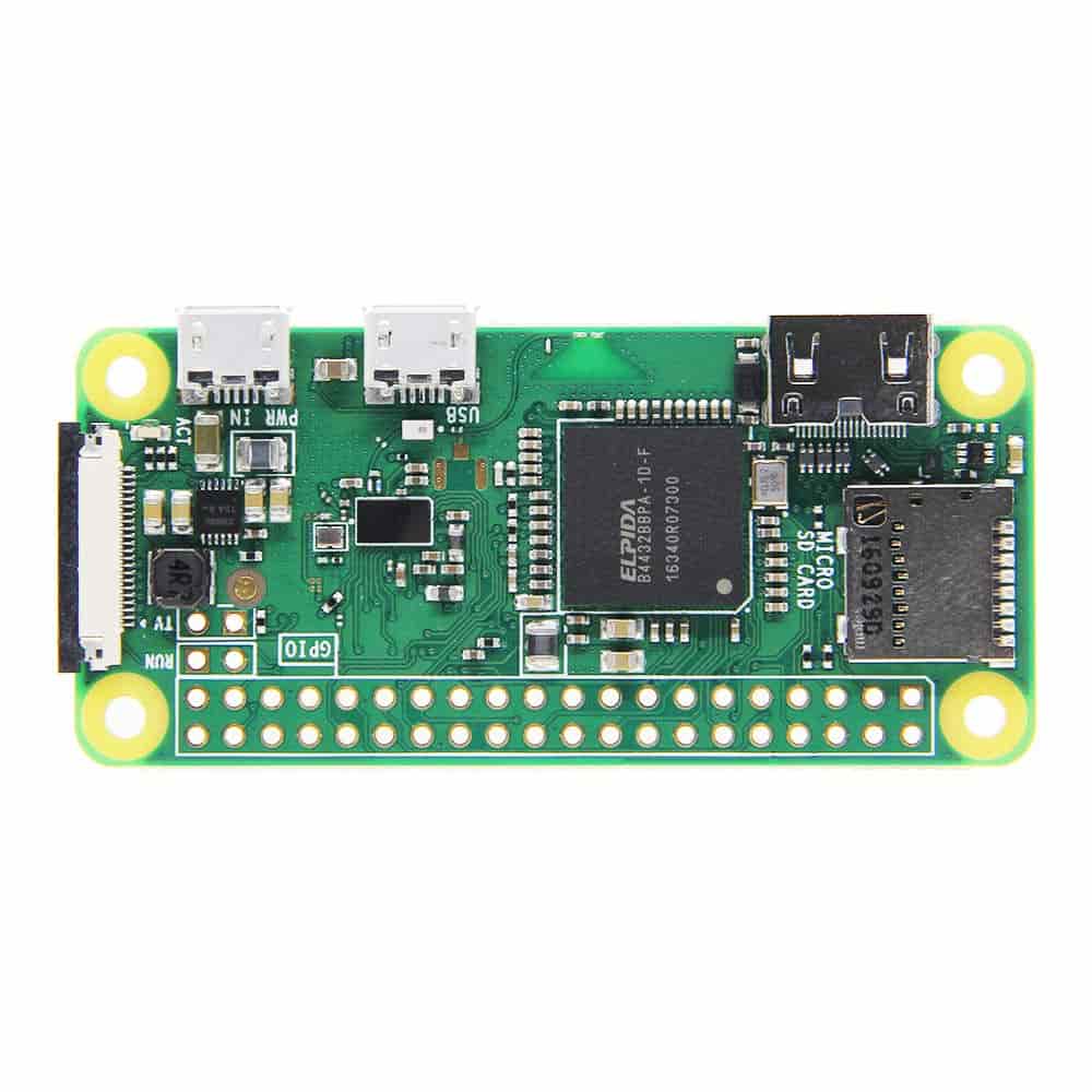
The Raspberry Pi Zero W is a compact, 65 mm × 30 mm ultra-low-power single-board computer. It features a 1GHz single-core CPU, 512MB RAM, and integrated 2.4GHz Wi-Fi and Bluetooth 4.1, making it ideal for IoT, robotics, and embedded DIY projects.

The Raspberry Pi Imager can be downloaded from:

https://www.raspberrypi.com/software/

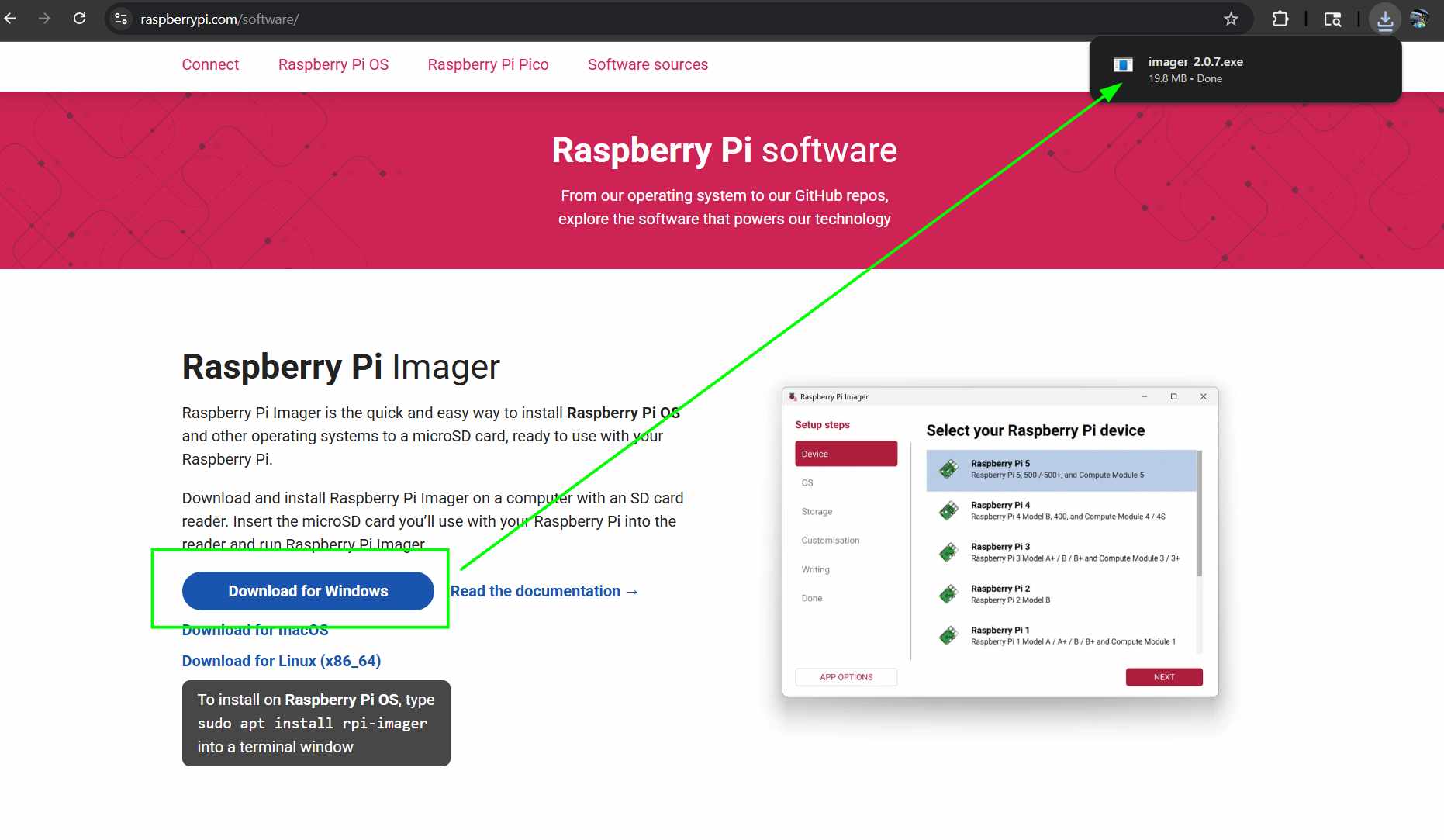
After installing the Raspberry Pi Imager, open the application.

Selecting the Raspberry Pi

The first screen asks which Raspberry Pi board will be used. For this project I selected the Raspberry Pi Zero W.

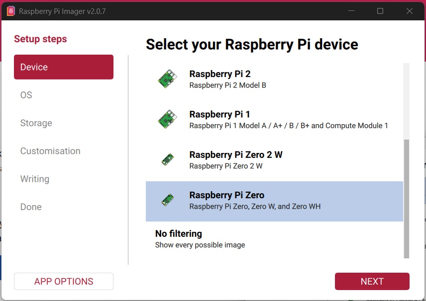
Although the Raspberry Pi Zero W has limited processing power compared to the newer Raspberry Pi boards, it is extremely compact, consumes very little power and is capable of running OpenCV for lightweight computer vision tasks.

Selecting the Operating System

Next the operating system needs to be selected.

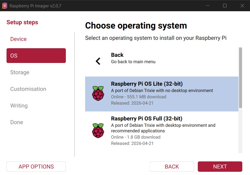
For this project I wanted a completely headless Raspberry Pi. No monitor, keyboard or mouse would ever be connected after flashing the SD card. Instead, all interaction would happen remotely over WiFi using SSH.

This allows the Pi Zero to remain mounted permanently inside the project while still allowing images to be captured using the camera with commands such as libcamera-still (or the newer rpicam-still) over an SSH connection.

Selecting the Storage Device

After selecting the operating system, choose the microSD card that will be used as the Raspberry Pi's storage device.

For the Raspberry Pi Zero W , a reputable 32GB A1 or A2 Class 10 microSD card is highly recommended. Top reliable options include the SanDisk Ultra, or Samsung EVO Plus.

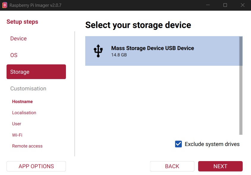
Everything required to boot the Raspberry Pi will be written onto this card, including the operating system and the custom configuration.

Customising the Raspberry Pi

Before writing the SD card, Raspberry Pi Imager allows the operating system to be customised.

I entered a hostname for the Raspberry Pi, choosing something simple such as pizero.

This hostname allows the Pi to later be accessed over the local network using addresses such as:

ssh pi@pizero.local

instead of remembering its IP address.

The localisation settings such as keyboard layout, timezone and WiFi region can also be configured at this stage.

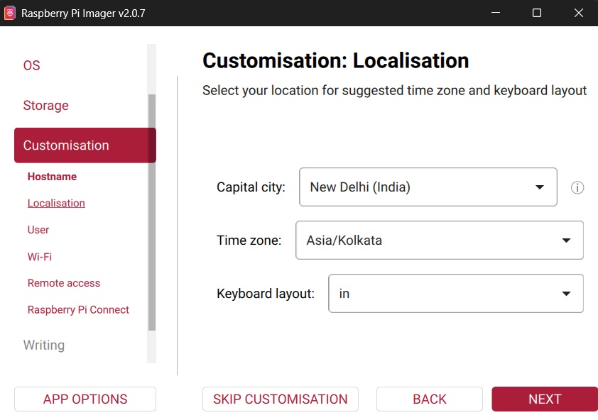
The final setup screen allows:

• Setting the Raspberry Pi username
• Creating a secure password
• Entering the WiFi SSID
• Entering the WiFi password
• Enabling SSH

Enabling SSH here is important because it allows the Raspberry Pi to be accessed remotely immediately after its first boot without requiring any peripherals.

Setting Up Headless SSH

You can follow this guide to set up headless SSH.

For a headless SSH connection to a Raspberry Pi Zero from Windows, I used Windows PowerShell.

Since this Raspberry Pi would never be connected to a monitor, enabling SSH during imaging was essential.

The process works as follows:

• The Raspberry Pi boots from the prepared microSD card.
• It automatically connects to the configured WiFi network.
• The SSH service starts automatically.
• The Pi advertises its hostname on the network using mDNS.
• Any computer connected to the same WiFi network can now connect to it.

On Windows I could then simply open PowerShell or Command Prompt and type:

ssh pi@pizero.local

The first connection asks whether the device should be trusted. After accepting the fingerprint, the password created earlier is entered and the terminal becomes fully connected to the Raspberry Pi.

Once connected, every command can be executed remotely exactly as though a keyboard and monitor were physically attached.

Writing the Operating System

After completing the configuration, the Raspberry Pi Imager writes the operating system to the microSD card.

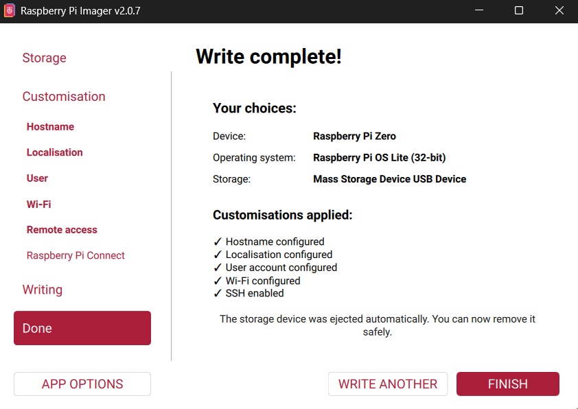
Once writing is complete, remove the SD card from the computer and insert it into the Raspberry Pi Zero W.

The Raspberry Pi can then be powered simply by connecting a micro USB cable to its power port.

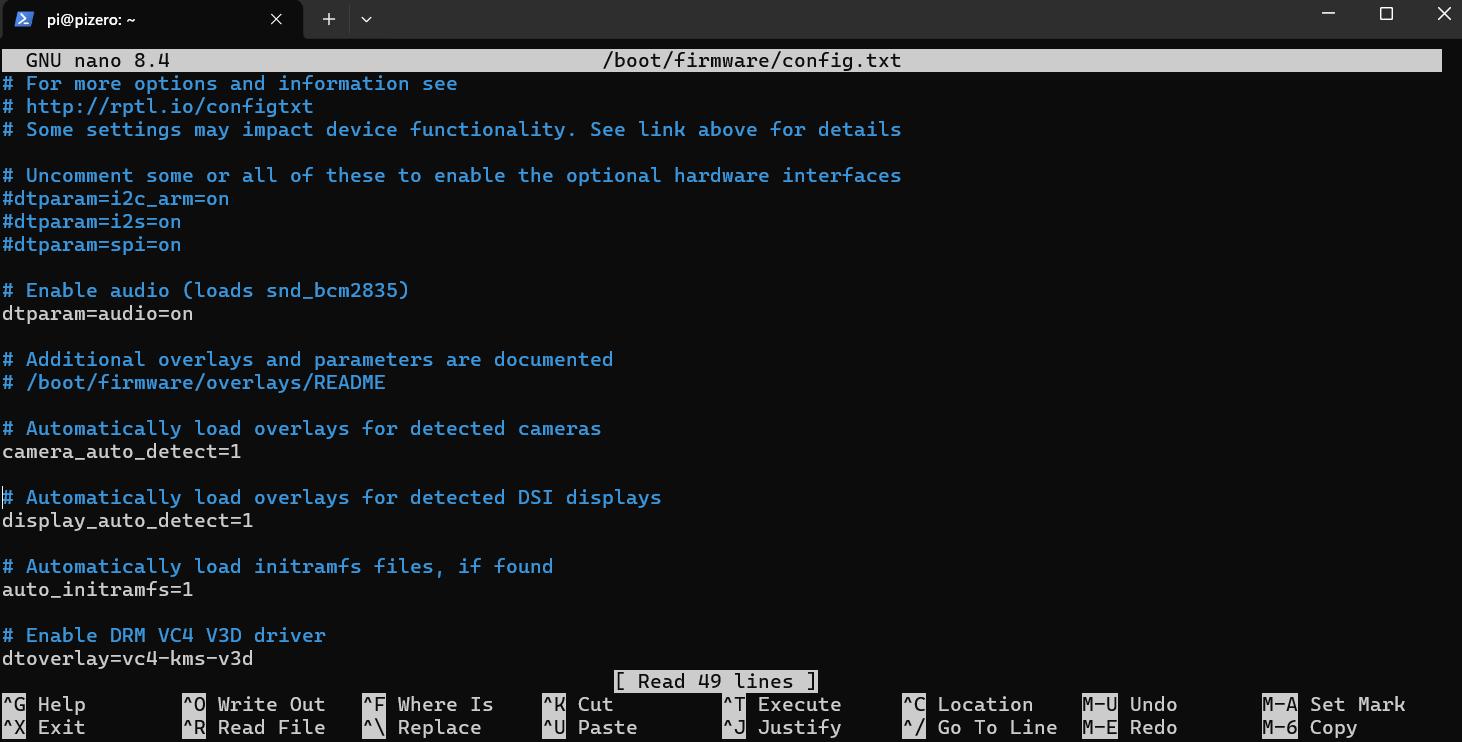
After approximately one minute the Raspberry Pi should automatically join the configured WiFi network and become accessible through SSH.

Installing Camera Software

The first package installed was the Raspberry Pi camera application package.

sudo apt update && sudo apt install -y libcamera-apps

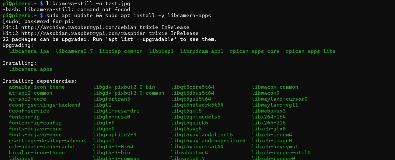
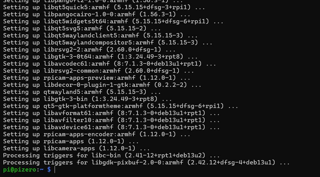
Recent Raspberry Pi OS releases have replaced libcamera-apps with rpicam-apps.

The functionality is effectively the same—the commands were simply renamed. For example:

• libcamera-still → rpicam-still
• libcamera-vid → rpicam-vid

These utilities provide access to image capture, video recording and camera configuration directly from the command line.

Installing Python and OpenCV

Since the image processing algorithms would be written in Python, Python 3 and pip were installed first.

sudo apt install python3 python3-pip -y

The project also required several scientific computing libraries.

• OpenCV for image processing
• NumPy for numerical array operations
• SciPy for signal processing and peak detection

First the package lists were updated:

sudo apt update

Then the required libraries were installed:

sudo apt install python3-numpy python3-opencv -y

If working on Windows instead, the equivalent installation command is:

py -m pip install opencv-python numpy

OpenCV provides the computer vision algorithms used throughout the project, while NumPy performs efficient matrix operations and SciPy provides functions such as signal smoothing and peak detection that are useful when analysing vinyl groove profiles.

Streaming Video

During development I often streamed live video directly from the Raspberry Pi instead of repeatedly capturing still images.

The TCP stream could be opened using:

tcp/h264://pizero.local:8888

Streaming the live camera feed made it much easier to adjust focus, camera height and lighting conditions while developing the groove detection algorithms.

Developing the Detection Algorithm

To speed up development I experimented with several Python scripts generated with the assistance of both ChatGPT and Claude.

Although each implementation differed slightly, they all generally followed the same computer vision pipeline:

• Detect the vinyl record.
• Mask only the groove region.
• Convert the circular grooves into a linear representation.
• Analyse brightness changes.
• Detect groove boundaries.
• Overlay the detected grooves back onto the original image for verification.

Cameras Used

To evaluate which camera would be better suited for groove detection, I tested two different Raspberry Pi camera modules.

• Raspberry Pi Camera Module Rev 1.3 (5 MP)
• Raspberry Pi Camera Module 3 (12 MP)

Both cameras were tested under similar lighting conditions using the same vinyl record so that the resulting images could be compared fairly.

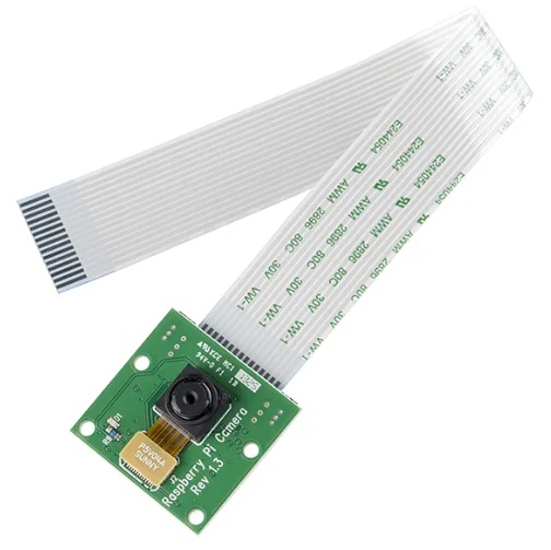
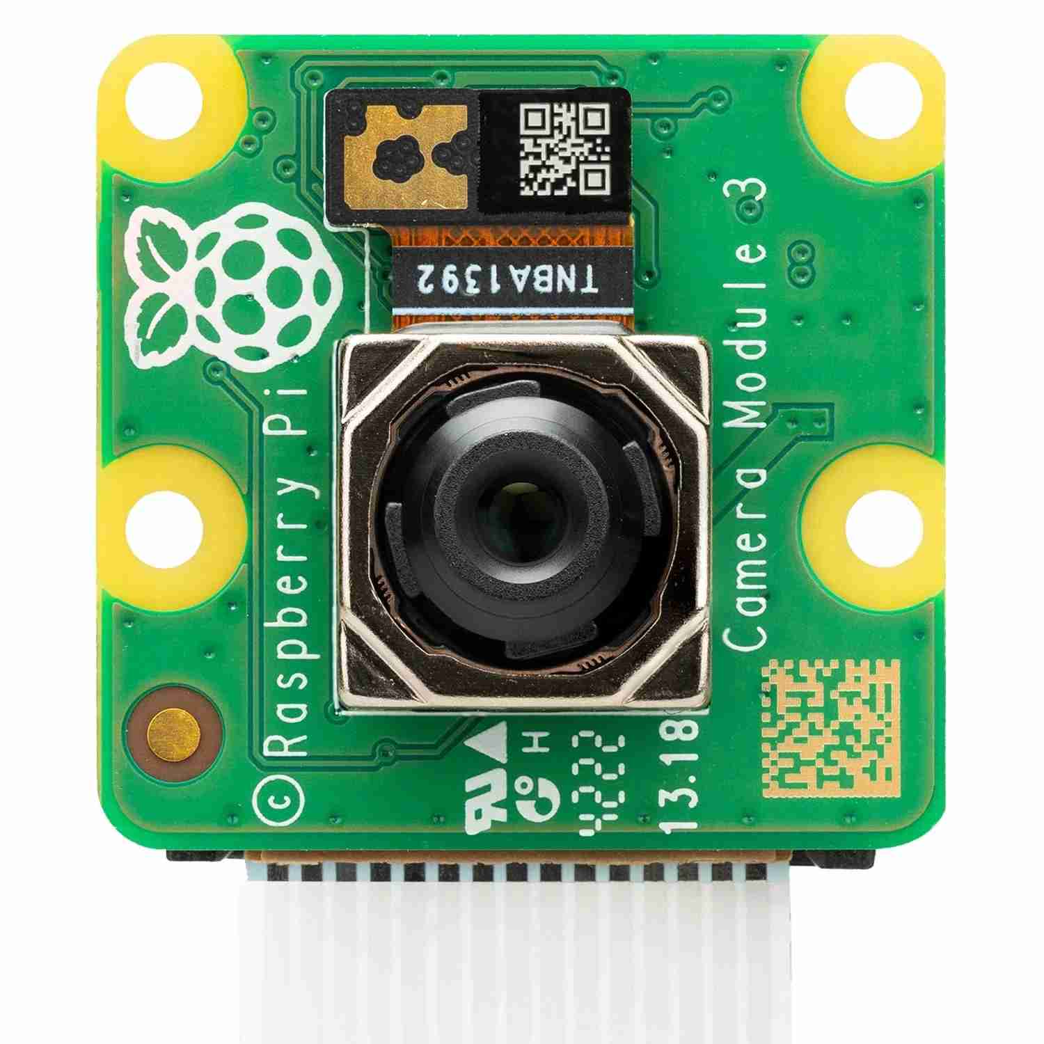
Front view of the camera module.

Camera Comparison

I made a rudimentary setup using a table lamp that we had at the soldering station. I did this so as to have consistent lighting.

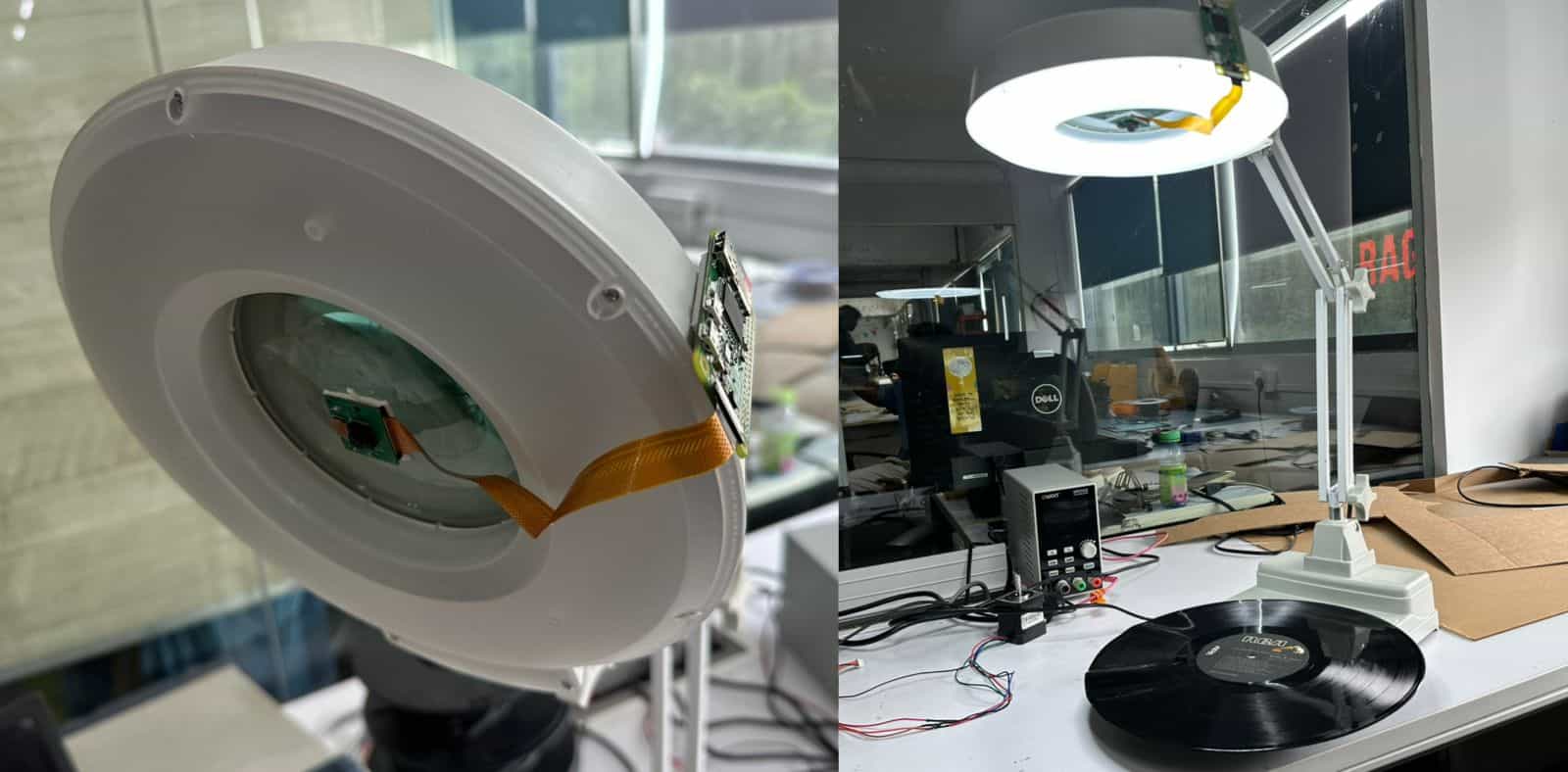
The record that I used for this test was The Best of Jim Reeves Volume III.

Both cameras produced promising images, although each had different strengths.

The older 5 MP Camera Rev 1.3 produced slightly softer images but provided a more gradual lighting transition across the vinyl surface. This smoother gradient made it easier to separate the darker groove bands from the surrounding material using simple thresholding techniques.

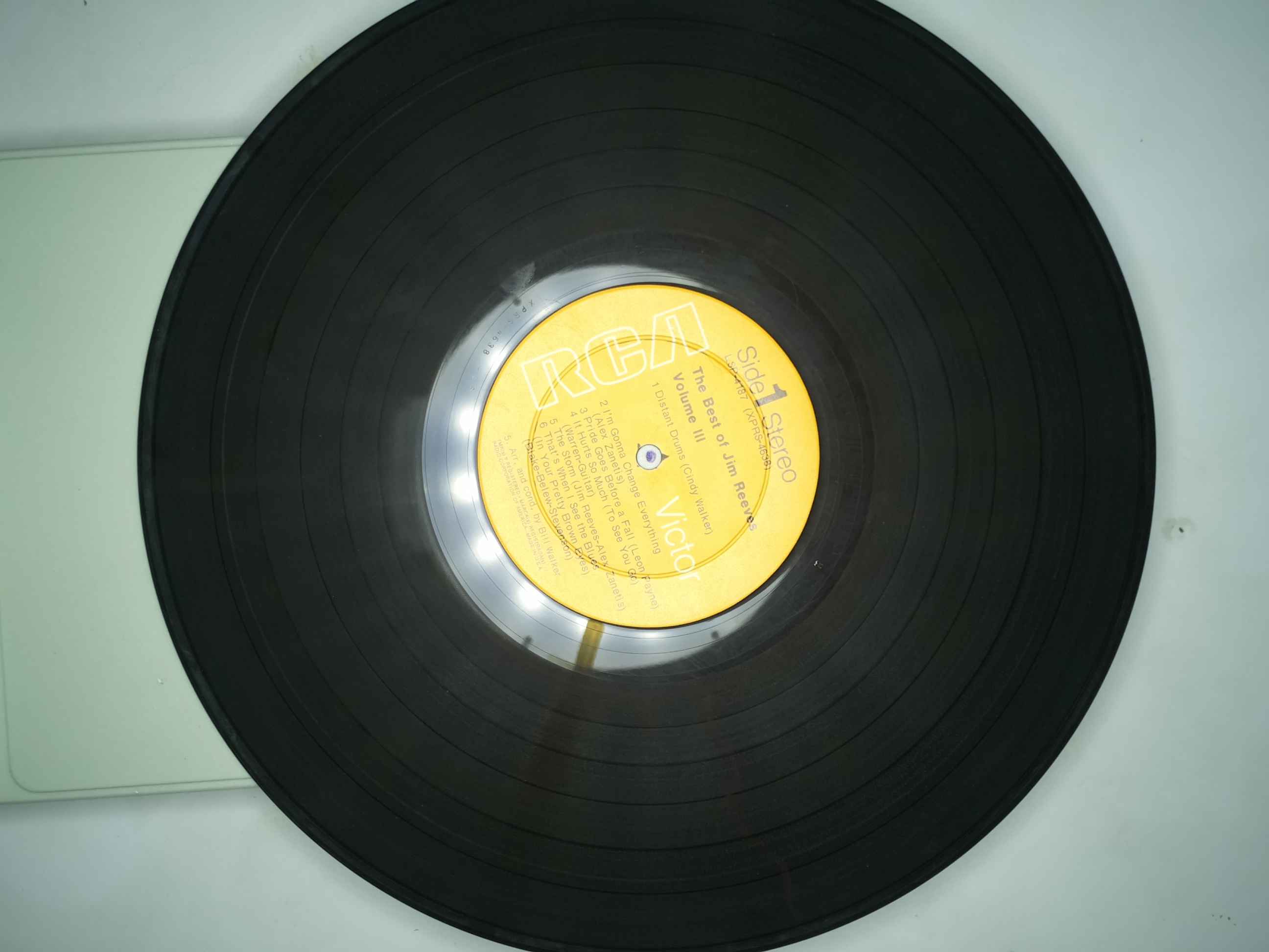
The newer 12 MP Camera Module 3 produced significantly sharper images with much higher detail. However, the increased resolution also captured far more small lighting variations and reflections, making the groove intensity less uniform across the record surface.

As a result, selecting a single threshold for groove detection became more challenging because the brightness varied considerably over the image.

Image captured using the Raspberry Pi Camera Rev 1.3.

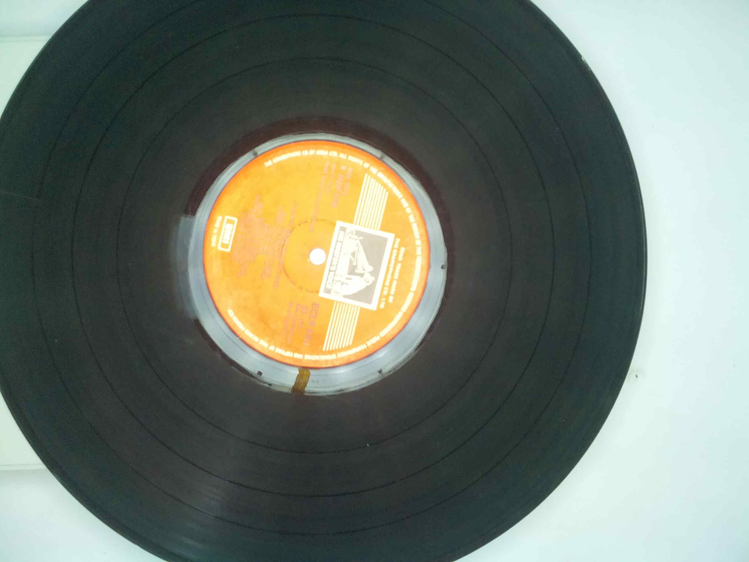
Image captured using the Raspberry Pi Camera Module 3.

Although the Rev 1.3 camera initially produced cleaner results for groove detection, I believe the Camera Module 3 has greater long-term potential. With more controlled lighting, a slightly different viewing angle and a diffused light source, the additional image resolution should allow much more accurate groove localisation.

Image Processing Pipeline

Although I generated several different versions of the Python code throughout the week, almost every implementation followed the same overall image processing pipeline.

The workflow consisted of five main stages:

1. Detect the vinyl record.
2. Mask only the groove region.
3. Convert the circular grooves into a polar representation.
4. Detect groove boundaries from the radial intensity profile.
5. Overlay the detected grooves back onto the original image.

Step 1 — Detecting the Record

The first task is locating the vinyl record within the captured image.

This was achieved using the Hough Circle Transform available in OpenCV. Because a vinyl record forms a nearly perfect circle, Hough Circle Detection is an effective method for estimating both the centre point and radius of the record.

The detected circle becomes the reference for every later processing step, since groove positions are always measured relative to the centre of the record.

Typical outputs from this stage are:

• Centre X coordinate
• Centre Y coordinate
• Outer record radius

Step 2 — Zone Masking

Once the record has been detected, only the region containing music grooves needs to be analysed.

Since a standard LP record is approximately 12 inches in diameter and the centre label occupies roughly the inner 4 inches, I can estimate where the grooves should exist without processing the entire image.

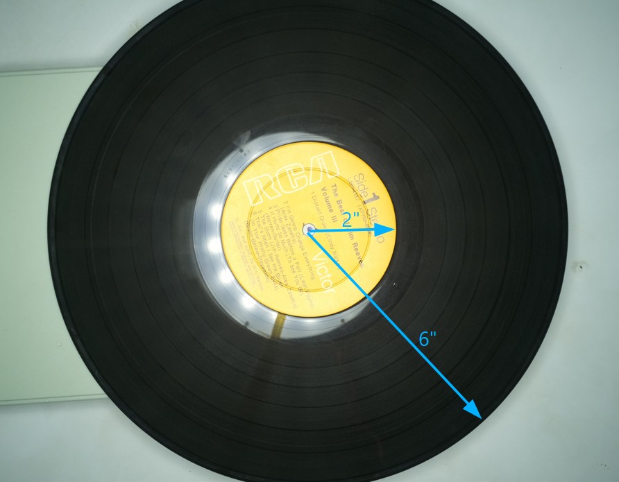
The highlighted annular region shown above represents the section used for groove detection.

Several additional margins are also introduced.

• The outer lead-in area is ignored.
• The centre label is ignored.
• A small inner margin skips the spill-off groove at the end of playback.

Restricting the analysis to only this region greatly reduces noise while also improving processing speed.

Step 3 — Polar Transformation

The next challenge is that vinyl grooves form concentric circles, making them difficult to analyse directly in Cartesian (X,Y) image coordinates.

Both ChatGPT and Claude independently generated approaches based around a polar coordinate transformation.

Instead of representing pixels using horizontal and vertical coordinates, the image is converted into radius and angle.

• X,Y coordinates become Radius, θ.
• Circular grooves become nearly horizontal lines.
• Analysing brightness along each ring becomes much easier.

This conversion effectively unwraps the circular vinyl record into a rectangular image where groove positions become almost straight horizontal bands.

An example of the transformed image is shown below.

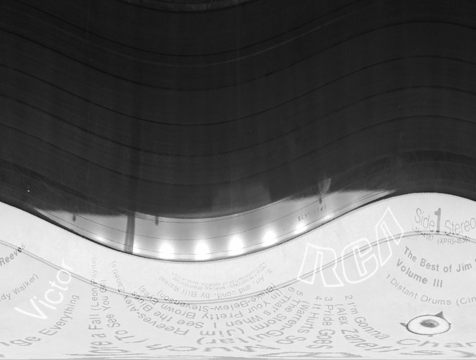
This representation simplifies later processing because image intensity can now be analysed one radius at a time instead of tracing complete circles.

Step 4 — Generating the Radial Brightness Profile

After converting to polar coordinates, the brightness of every circular ring is averaged around the full circumference.

This produces a one-dimensional graph where:

• X-axis = distance from the record centre.
• Y-axis = average brightness.

Instead of processing millions of image pixels individually, the algorithm now works with a simple brightness-versus-radius signal.

Whenever a groove exists, the groove walls appear darker than the surrounding vinyl surface.

These darker regions produce sudden drops in brightness, which appear as local minima within the radial intensity profile.

This significantly simplifies the groove detection process.

Step 5 — Peak Detection

The next stage analyses the one-dimensional radial profile to locate the groove boundaries.

Instead of searching for bright peaks, the algorithm searches for local minimum values because the grooves appear darker than the surrounding vinyl.

To avoid detecting the same groove multiple times, the scripts also applied an adaptive minimum spacing between neighbouring peaks.

This prevents tiny fluctuations caused by noise from being interpreted as additional grooves.

The resulting radial profile is shown below.

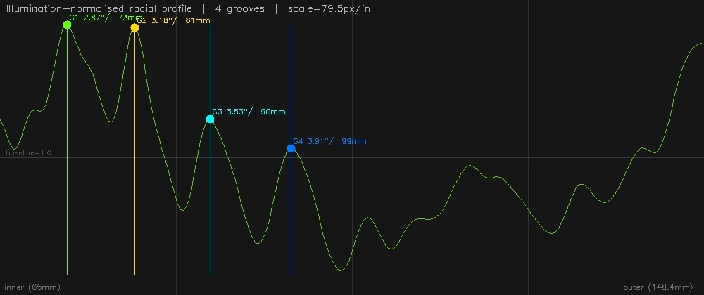
Each major dip in the graph corresponds to one groove wall or one large groove transition.

These detected positions can then be converted back into circular coordinates on the original image.

Step 6 — Cartesian Overlay

The final processing stage converts the detected groove positions back from polar coordinates into the original image.

This overlay provides a simple visual verification of whether the algorithm is correctly identifying groove locations.

If the detected circles align with the visible groove bands on the vinyl record, the processing pipeline is behaving as expected.

Throughout the week I generated several different versions of this algorithm, gradually improving the groove localisation.

Algorithm Development

The progression of the algorithm, including its development, iterations, and refinements, can be found in the Claude chat linked here.

Throughout the week I generated and tested several different versions of the groove detection algorithm. Each version attempted to improve the accuracy of groove localisation while reducing false detections caused by reflections, surface scratches and lighting variations.

Although every version followed the same overall processing pipeline, the parameters and processing methods were gradually refined based on the results from previous attempts.

Running the Script Headlessly

The Python script was transferred to the Raspberry Pi Zero over SSH using the scp command from Windows. After copying the file, an SSH session was opened to the Pi, where the script was executed using Python.

1. Power the Raspberry Pi Zero and ensure it is connected to the same network as the computer.
2. Open a terminal on the computer and connect to the Pi:

   ssh pi@raspberrypi.local

3. Transfer the Python script to the Pi:

   scp groove_detector.py pi@raspberrypi.local:~

4. Log in to the Pi and run the script:

   python3 groove_detector.py

Captured Images

The camera captures and saves images in the same directory as the Python script unless a different save path is specified in the code.

Copying Images Back to the Computer

From the computer, use scp to copy the captured image:

scp pi@raspberrypi.local:~/captured_image.jpg .

This copies captured_image.jpg from the Raspberry Pi to the current folder on the computer. Replace the filename with the appropriate output image if necessary.

First Implementation

Prompt Used

I have images of vinyl records captured using a Raspberry Pi camera.
The grooves appear as concentric circular dark/light patterns.
I want an optimized Python OpenCV pipeline to detect and visualize the grooves.
Requirements:
1. Automatically detect the record center using Hough Circle Transform.
2. Convert the image from Cartesian coordinates to polar coordinates so the grooves become horizontal lines.
3. Enhance groove visibility using:
   - CLAHE contrast enhancement
   - illumination normalization
4. Extract grooves using a combination of:
   - high-pass filtering
   - Sobel filtering in radial direction
   - optional Gabor filtering tuned for horizontal textures
5. Apply adaptive thresholding to isolate grooves.
6. Optionally convert the detected grooves back into Cartesian coordinates.
7. Code must run efficiently on a Raspberry Pi Zero W.
8. Provide well-structured modular Python code with comments.
9. Include parameter tuning guidance.
Important:
Do NOT use basic edge detection alone.
Exploit the circular symmetry of vinyl grooves using polar transforms.

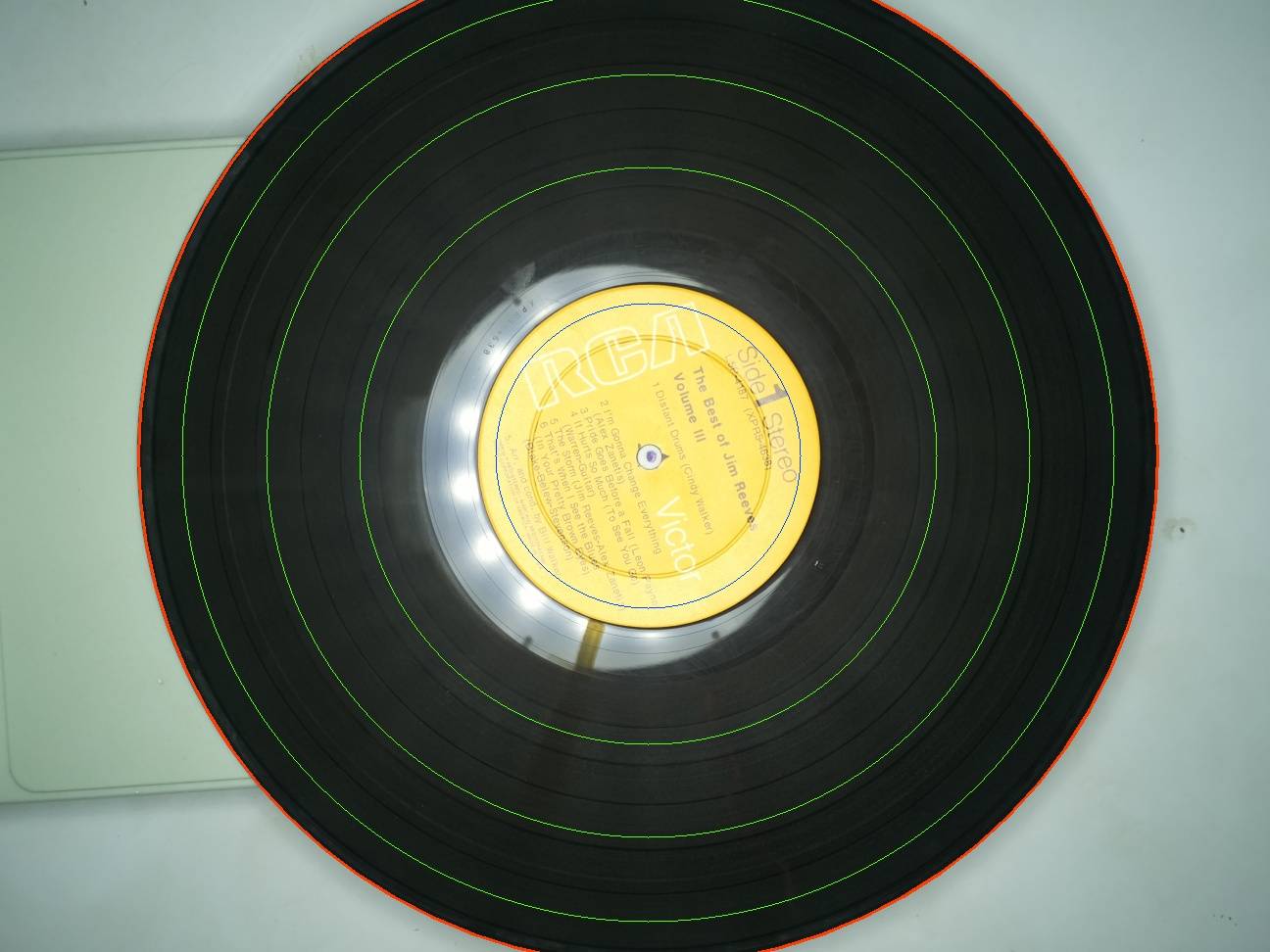
The first version of the algorithm simply detected the vinyl record, converted it into polar coordinates and attempted to detect grooves directly from the radial brightness profile.

The overall concept worked well, however the script analysed the entire record surface, including regions that would never contain usable groove information.

This resulted in several false detections around the outer lead-in groove and the inner run-out area.

Cartesian overlay generated by the first version.

Resulting radial profile.

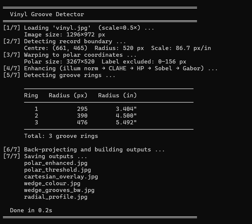
The first version demonstrated that the overall workflow was viable, but it became clear that limiting the region of interest would greatly improve the results.

Version 1

Prompt Used

This is the code right now, and I'm getting groove detection like this. Fix the code so that it can detect the grooves better.

Also, one thing that can be done for improvement is that the outer diameter is already being detected nicely. Since it is a 12-inch record, use that to determine the center of the record. The center label is 4 inches (about 100 mm) in diameter, and there is also a spill-off region where there are no grooves that extends about 15 mm radially beyond the label. So grooves should only be detected outside a 130 mm diameter circle. Adjust the code so this is implemented for better groove detection.

Also, in this image there are actually 4 grooves from the outside. The first one was missed, the second one was detected, and the third and fourth were missed. From the outer radius there is also about 4 mm of radial spill-off where there are no grooves, so only detect grooves between the 130 mm diameter inner boundary and 4 mm inside the detected outer radius.

Keep the existing detection approach as much as possible and improve it rather than replacing it. Update and check the `.md` file as well, and provide the complete updated `.py` and `.md` files.

The first major improvement was introducing boundaries so that only the playback area of the record would be analysed.

Instead of processing the complete radius of the record, the algorithm now restricted itself to the region between the lead-in groove and the centre label.

Additional functions were also introduced to calculate the groove radius more accurately relative to the detected centre of the record.

Although this significantly reduced unwanted detections, the groove positions were still not sufficiently accurate.

The algorithm occasionally drifted away from the correct groove locations, especially towards the inner portion of the record.

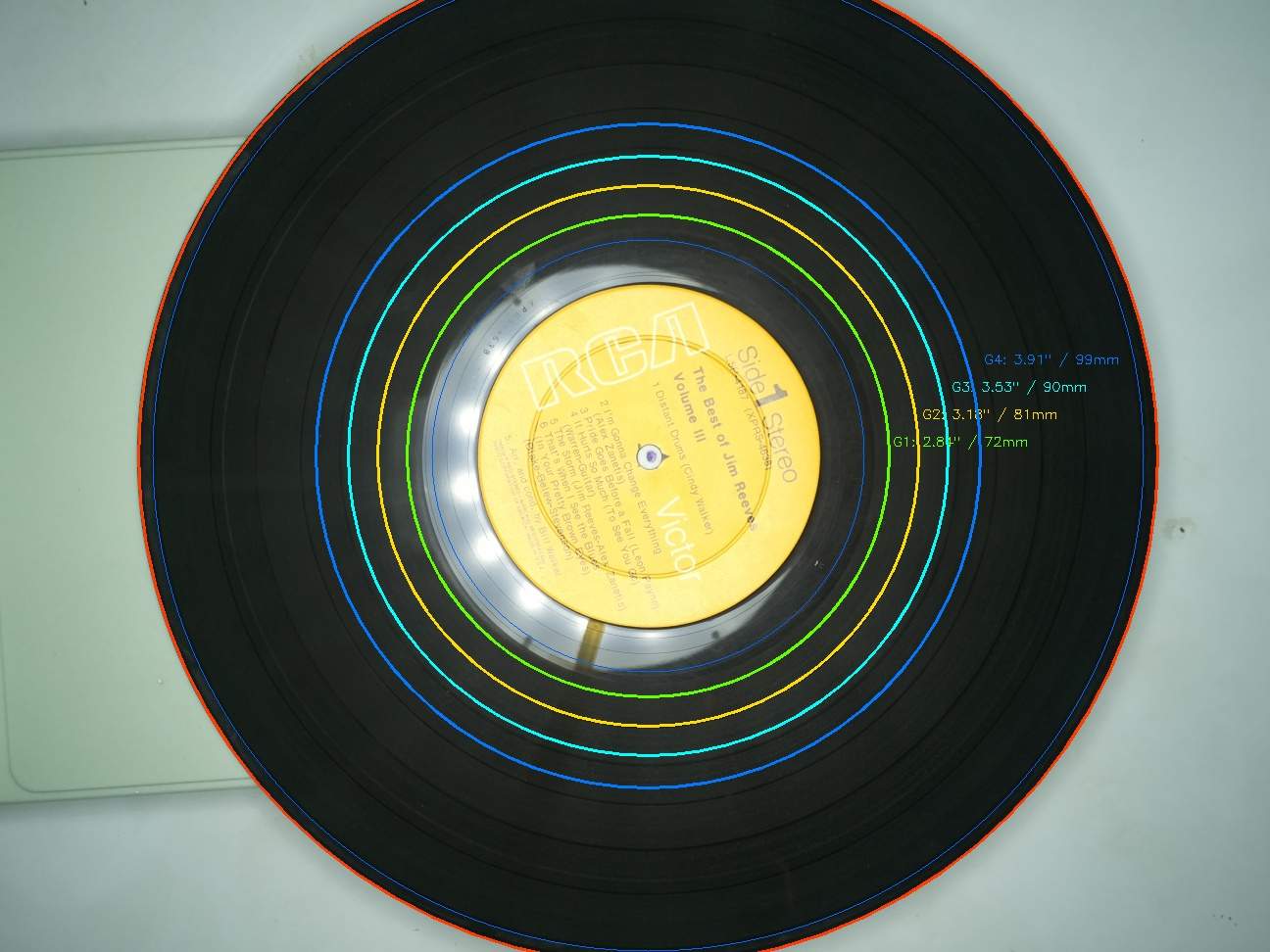
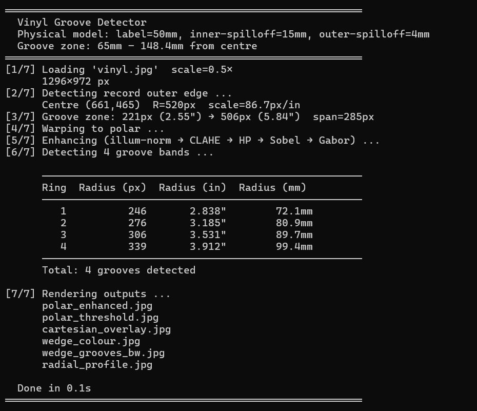
At this stage the algorithm was correctly detecting many of the groove transitions but still required considerable refinement before it could be used reliably.

Version 2

Prompt Used

  Coming like this now, but in the wedges I can clearly see the groove edges. Use the constraints that were discussed before (outer diameter, center label, inner spill-off, and outer spill-off) to limit the search region, and then search for the grooves using the same peak detection logic from the previous code I gave instead of changing the detection method.

The grooves are clearly visible in the wedge images, so analyze why the current implementation is missing them. Tune the preprocessing and the peak detection parameters so the grooves are detected consistently. Keep the existing approach as much as possible, improve it rather than replacing it, update the `.md` file to reflect the changes, and provide the complete updated `.py` and `.md` files.

The second version focused primarily on parameter tuning rather than changing the overall algorithm.

Several OpenCV parameters were adjusted to improve the robustness of the detection process.

Some of the parameters that were experimented with included:

• Gaussian blur kernel size to reduce image noise.
• Hough Circle sensitivity for more consistent record detection.
• Minimum and maximum record radius limits.
• Threshold values used when detecting darker groove bands.
• Peak prominence used during radial profile analysis.
• Minimum peak spacing to prevent multiple detections of the same groove.
• Brightness smoothing applied before peak detection.

Each parameter had a noticeable influence on the final groove positions. Finding a combination that worked consistently across different vinyl records proved to be considerably more challenging than expected because lighting conditions varied from image to image.

Output generated by Version 2.

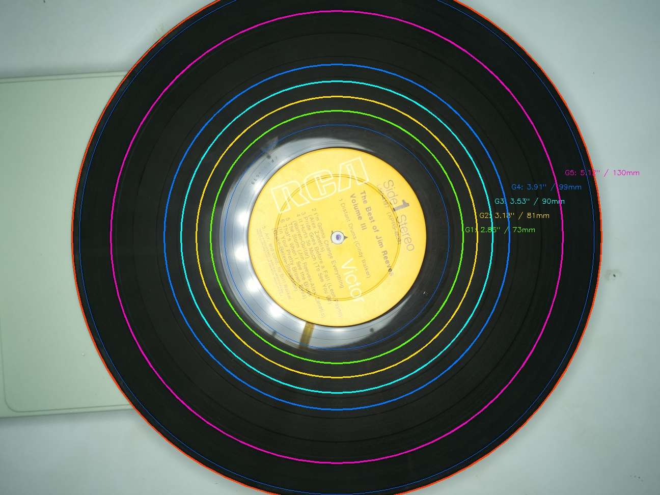
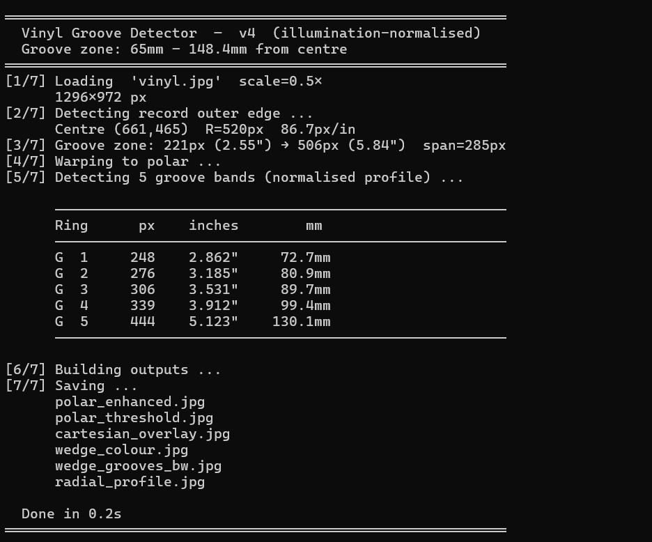
Version 2 produced more stable groove counts than the previous version, although the detected groove positions were still slightly offset from their actual locations.

Version 3

Prompt Used

If a Raspberry Pi camera captures an image like this, I want to locate the number of tracks on the vinyl record for a project that can automatically position the tonearm over any selected track after detecting the record's location using the Pi camera.

Use the known geometry of a standard 12-inch record to improve detection. The total diameter is 12 inches, and the center label is approximately 4 inches (100 mm) in diameter. Grooves only exist outside the center label, and there is an additional spill-off region around the label where no grooves are present. Likewise, there is a spill-off region near the outer edge of the record where no grooves exist.

The first dark band closest to the outside of the record marks the beginning of the first track and should be treated as Track 1. The last thick dark band near the center is the run-out/spill-off region and should never be counted as a track. Every valid groove boundary between these two regions should be detected and counted as a track.

I want an OpenCV-based Python script that is robust enough to handle images captured by a Raspberry Pi camera under realistic lighting conditions. The script should first detect the record and its center, use the known record dimensions to restrict the search to the valid groove region, unwrap the groove area if necessary, detect the groove boundaries reliably, count all tracks accurately, and visualize the detected tracks on the output image for debugging. Please explain the approach, update the documentation if needed, and provide the complete working Python code.

For the third version I decided to generate a completely new implementation using Claude rather than continuing to modify the previous scripts.

The progression of the algorithm, including its development, iterations, and refinements, can be found in the Claude chat linked here.

Although the overall processing stages remained similar, the internal implementation was considerably different.

The newer algorithm produced much cleaner radial profiles and significantly improved groove localisation.

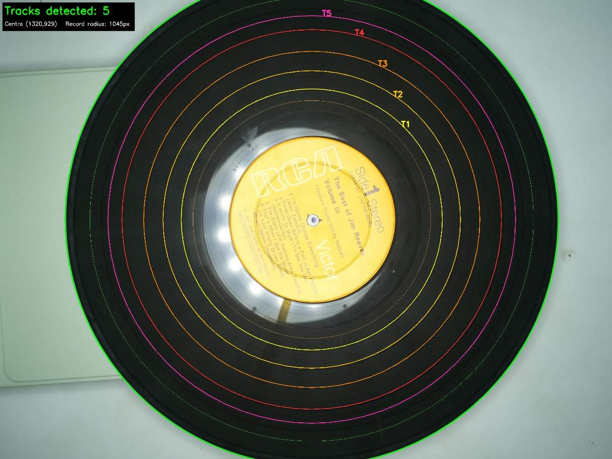
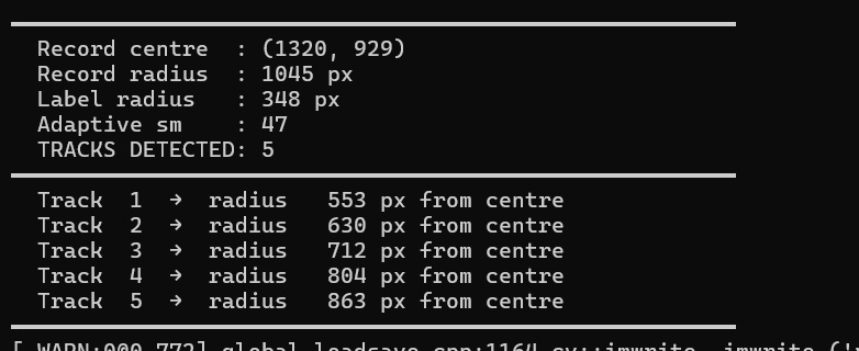
This version represented the closest result obtained during the week. Most groove boundaries were being detected correctly and the overall groove count closely matched the physical record.

Additional Testing

To determine whether the algorithm would generalise beyond a single vinyl record, I repeated the testing process using several different records with different groove spacing, colours and surface conditions.

The newer Version 3 algorithm consistently detected approximately the correct number of groove bands across multiple records.

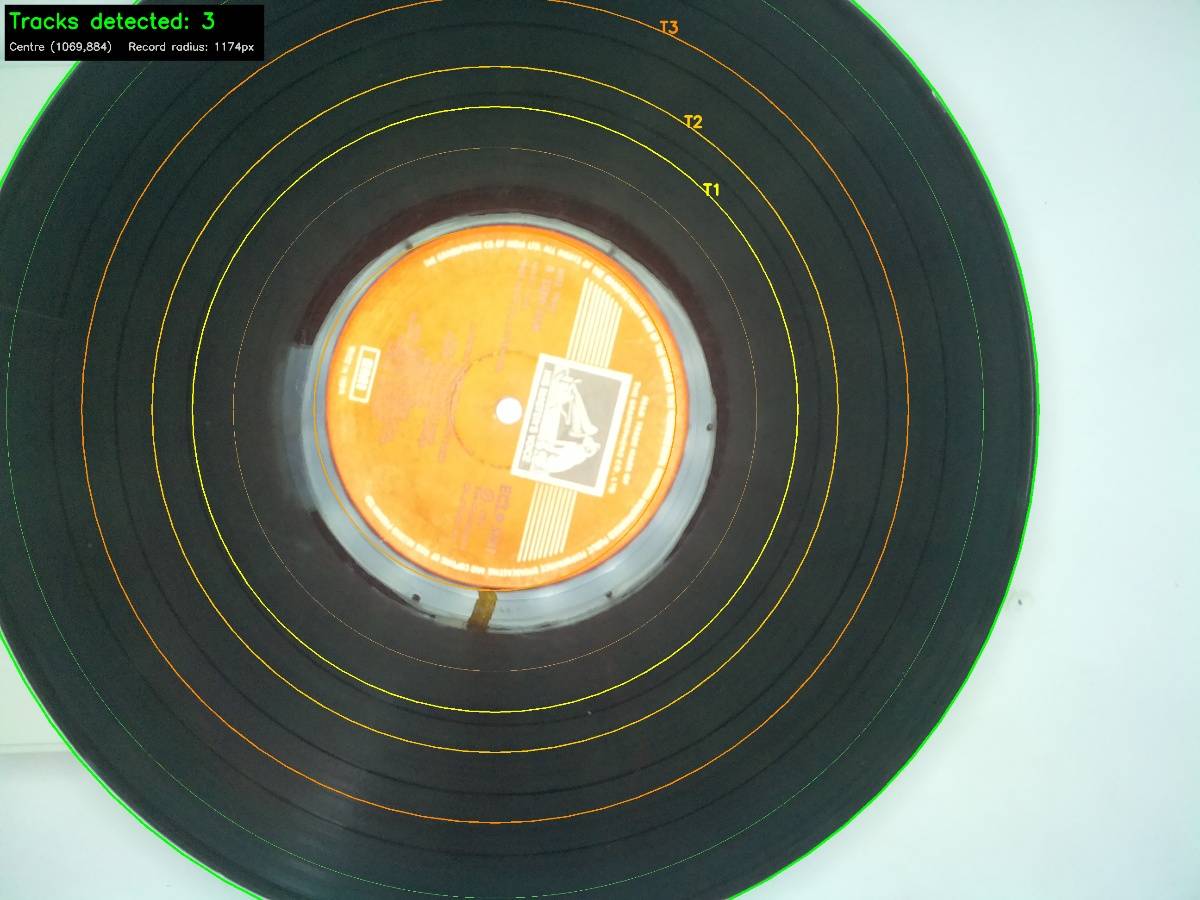
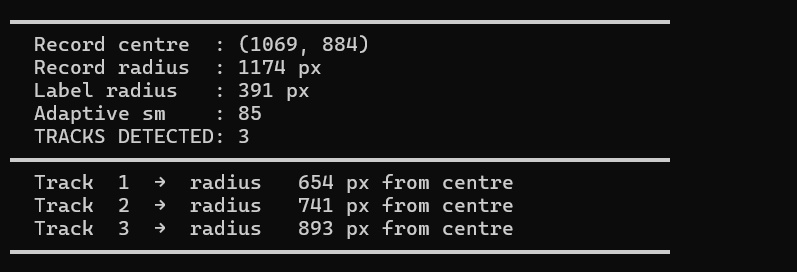
Although the groove count was encouraging, the exact groove positions still required further refinement.

Some detected grooves appeared slightly shifted from their true locations, particularly near the centre of the record where the grooves become more closely spaced.

Current Results

The final tests carried out during the week produced the correct groove count on several records, however the groove positions were still not perfectly aligned with the actual groove bands.

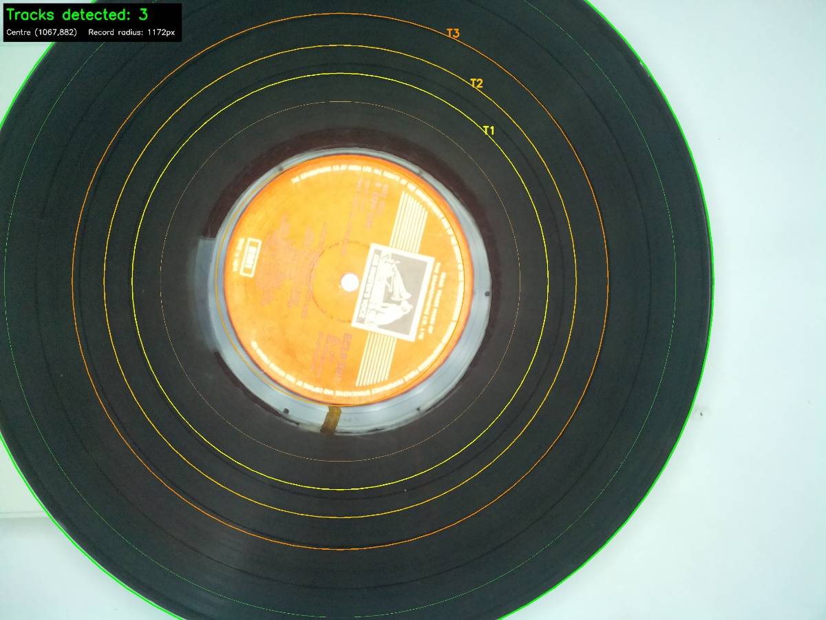
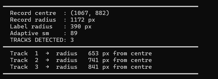
At this stage the algorithm successfully demonstrates that automatic groove detection using a Raspberry Pi and OpenCV is achievable.

Future work will focus on improving the positional accuracy of the detected grooves by:

• Improving the lighting setup using more diffuse illumination.
• Experimenting with different camera heights and viewing angles.
• Further tuning the peak detection parameters.
• Testing adaptive thresholding instead of fixed thresholds.
• Improving polar image preprocessing before groove extraction.
• Testing additional filtering techniques to suppress reflections.

Conclusion

Although the groove detection system is still under development, the progress made during Wildcard Week established a strong foundation for the remainder of the project. The Raspberry Pi Zero W proved capable of running OpenCV-based image processing, while both Raspberry Pi camera modules produced images of sufficient quality for experimentation.

The most significant outcome of the week was demonstrating that groove positions can be estimated automatically using computer vision techniques. While further improvements are still required before the system can reliably identify the exact beginning of every song, the current implementation already detects the correct number of groove transitions on many records and provides a promising basis for fully automated track selection in the final project.

Project Files