Software & Tools


Python Interfacing with Microcontrollers
This documentation covers the Jupyter Notebook interface-and-application-programming.ipynb, which demonstrates how to connect a microcontroller to Python running on a host computer — starting with a raw serial read and progressively building up to a real-time 3D web visualization driven by a physical potentiometer.
Download File: For the clearest view of the complete code, use the downloads in the Project Files section. The downloadable notebook and companion files make the full source easier to inspect, while the .ipynb itself is intentionally structured as a clean, readable file for working along step by step.
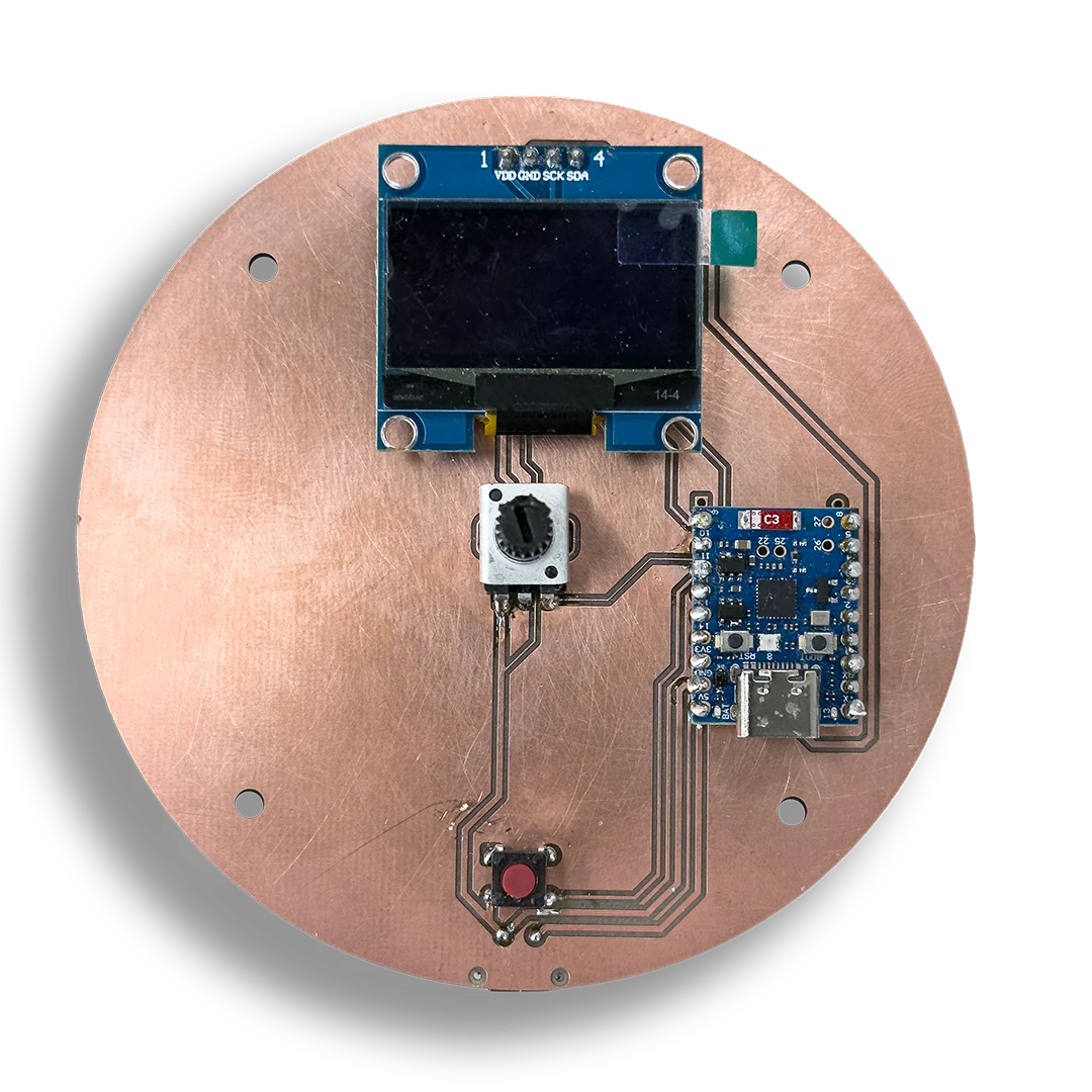
The hardware used is an ESP32-C6 Super Mini with a potentiometer connected to GPIO 5. As you turn the potentiometer, an ADC (Analog-to-Digital Converter) reads the voltage and sends it as a number over USB to the computer. Python receives that number and does something useful with it.
The notebook introduces the software stack step by step: pyserial handles the USB serial data, tkinter creates desktop UI windows, matplotlib turns readings into live plots, FastAPI and uvicorn bridge the data into a WebSocket, websockets helps with debugging, and three.js renders the browser-based 3D visualization.
Setup
Project Structure
The download ZIP contains three things: a venv folder with all Python dependencies pre-installed, a notebooks folder with the Jupyter Notebook and all companion scripts, and a requirements.txt file listing the dependencies. The companion scripts are small standalone Python files that get launched from within the notebook — they exist separately because some of them open blocking windows that would freeze the Jupyter kernel if run directly in a cell.
venv/
notebooks/
    interface-and-application-programming.ipynb
    simple-tkwindow.py
    poti-monitor.py
    poti-realtime-plot.py
    poti-adc-noise.py
    server.py
    poti-threejs.html
requirements.txt
Activating the Virtual Environment
Open a terminal in the project root and activate the virtual environment before starting Jupyter.
On Windows, run:
venv\Scripts\activateOn macOS or Linux, run:
source venv/bin/activateThen start Jupyter with:
jupyter notebookYou should see (venv) appear at the beginning of the terminal prompt, confirming the environment is active. Open interface-and-application-programming.ipynb from the browser interface that appears.
Hardware & Firmware
Hardware Setup
Connect a potentiometer to the ESP32 as follows: one outer pin goes to 3.3V, the other outer pin goes to GND, and the middle wiper pin connects to GPIO 5. Then connect the ESP32 to your computer via USB.
If you are using a Chinese ESP32 Super Mini (the small board with the castellated edges), you need to enable USB CDC on Boot in the Arduino IDE under Tools before flashing. Without this setting, the board will not send any data over the serial connection and the notebook will receive nothing.
To find the correct port, open Device Manager on Windows and look under "Ports (COM & LPT)" — you will see something like COM5. On macOS or Linux, run ls /dev/tty.* in the terminal. Update the port string in the notebook cells to match your system. The default in the notebook is "COM5".
ESP32 Firmware
Before running the notebook, flash the following sketch to your ESP32 using the Arduino IDE:
The sketch reads the raw ADC value from GPIO 5 every 100 milliseconds and prints it as a plain integer over the serial connection at 115200 baud. The 12-bit resolution means values range from 0 to 4095 in theory, though in practice the usable range depends on the potentiometer and board tolerances — around 0 to 3168 was observed during testing.
const int POTI_PIN = 5;

void setup() {
  Serial.begin(115200);
  analogReadResolution(12);
}

void loop() {
  int raw = analogRead(POTI_PIN);
  Serial.println(raw);
  delay(100);
}
Notebook Walkthrough
Reading Serial Data
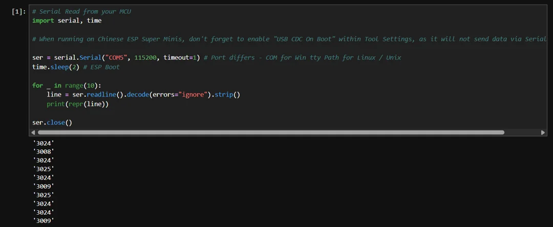
This is the most fundamental step: opening a connection to the ESP32 and reading ten lines of raw data. The serial.Serial() call opens the port at 115200 baud, which must match the baud rate set in the firmware. The timeout=1 parameter tells readline to wait at most one second for a line before returning, which prevents the script from hanging indefinitely if no data arrives.
The time.sleep(2) pause after opening the port is important — the ESP32 reboots when a serial connection is established, and it takes a moment to finish booting and start sending data. Without this pause, the first few reads would likely return empty strings.
Once a line arrives, it is a raw bytes object. The .decode() call converts it to a Python string, and .strip() removes the trailing newline character. Wrapping it in repr() when printing shows the quotes around the value, making it easy to confirm the data looks exactly as expected — for example '2640' rather than just 2640. After reading ten values, ser.close() releases the port so it is available for the next cell.
# Serial Read from your MCU
import serial, time

# When running on Chinese ESP Super Minis, don't forget to enable "USB CDC On Boot" within Tool Settings, as it will not send data via Serial otherwise

ser = serial.Serial("COM5", 115200, timeout=1) # Port differs - COM for Win tty Path for Linux / Unix
time.sleep(2) # ESP Boot

for _ in range(10):
    line = ser.readline().decode(errors="ignore").strip()
    print(repr(line))

ser.close()
Simple Tkinter Window
This step uses a small companion script that opens a basic desktop window with a "Hello World!" label. The actual code is straightforward Tkinter: create a root window, add a label, call mainloop(). Because Tkinter's mainloop() is blocking, the runnable notebook keeps it in a separate file. On this page, the full script is shown directly instead of the notebook launcher so the implementation is easier to read.
import tkinter as tk

root = tk.Tk()
root.title("Simple Window")

label = tk.Label(root, text="Hello World!", font=("Arial", 24))
label.pack(padx=40, pady=40)

root.mainloop()
Live Potentiometer Monitor
This cell combines the serial reader from Cell 1 with the Tkinter window from Cell 2. The companion script poti-monitor.py opens a desktop window that displays the current potentiometer value, updating every 50 milliseconds as you turn the dial.
The most important design decision in this script is setting timeout=0 when opening the serial port. A blocking timeout would cause readline() to pause for up to a second waiting for data, which would make the Tkinter window freeze and feel unresponsive. With timeout=0, readline() returns immediately with whatever data is available, and the window stays fluid.
The update loop is implemented using root.after(50, update), which tells Tkinter's event loop to call the update function again after 50 ms. This cooperates with the GUI framework rather than fighting it — a plain while loop would block the event loop entirely and crash the window. The line.isdigit() check filters out any malformed or empty lines before updating the label, ensuring only valid integers are displayed.
The close-handling pattern safely releases any previously open serial connection. This is important throughout the notebook because cells are often re-run, and attempting to open a port that is already open raises an error.
import tkinter as tk
import serial

ser = serial.Serial("COM5", 115200, timeout=0)  # timeout=0 = non-blocking!

def update():
    line = ser.readline().decode(errors="ignore").strip()
    if line.isdigit():
        label.config(text=f"Poti Value: {line}")
    root.after(50, update)

def on_close():
    ser.close()
    root.destroy()

root = tk.Tk()
root.title("Poti Monitor")

label = tk.Label(root, text="Poti Value: –", font=("Arial", 24))
label.pack(padx=40, pady=40)

root.protocol("WM_DELETE_WINDOW", on_close)

update()
root.mainloop()
Reading and Plotting Values
This cell moves beyond displaying a single value and instead collects a series of ten measurements, then plots them as a line chart directly inside the notebook. The chart makes patterns immediately visible that would be hard to notice from individual numbers — things like noise, drift, or sudden jumps when the potentiometer is moved.
The safe open pattern here is explicit: the try/except first closes any lingering connection, then a fresh ser = serial.Serial(...) always opens a new one. This is more reliable than trying to detect whether the port is already open, particularly after kernel restarts.
#This reads 10 of the serial values, prints them and then plots them using matplotlib library
import serial, time
import matplotlib.pyplot as plt

try:
    ser.close()
except Exception:
    pass

# Serial Open and Read 10 Values
ser = serial.Serial("COM5", 115200, timeout=1)
time.sleep(2)


time.sleep(2)

values = []
for _ in range(10):
    line = ser.readline().decode(errors="ignore").strip()
    if line.isdigit():
        values.append(int(line))

ser.close()
print(values)

# Plot Poti Values
plt.plot(values)
plt.title("Poti Values")
plt.ylabel("ADC")
plt.xlabel("Sample")
plt.show()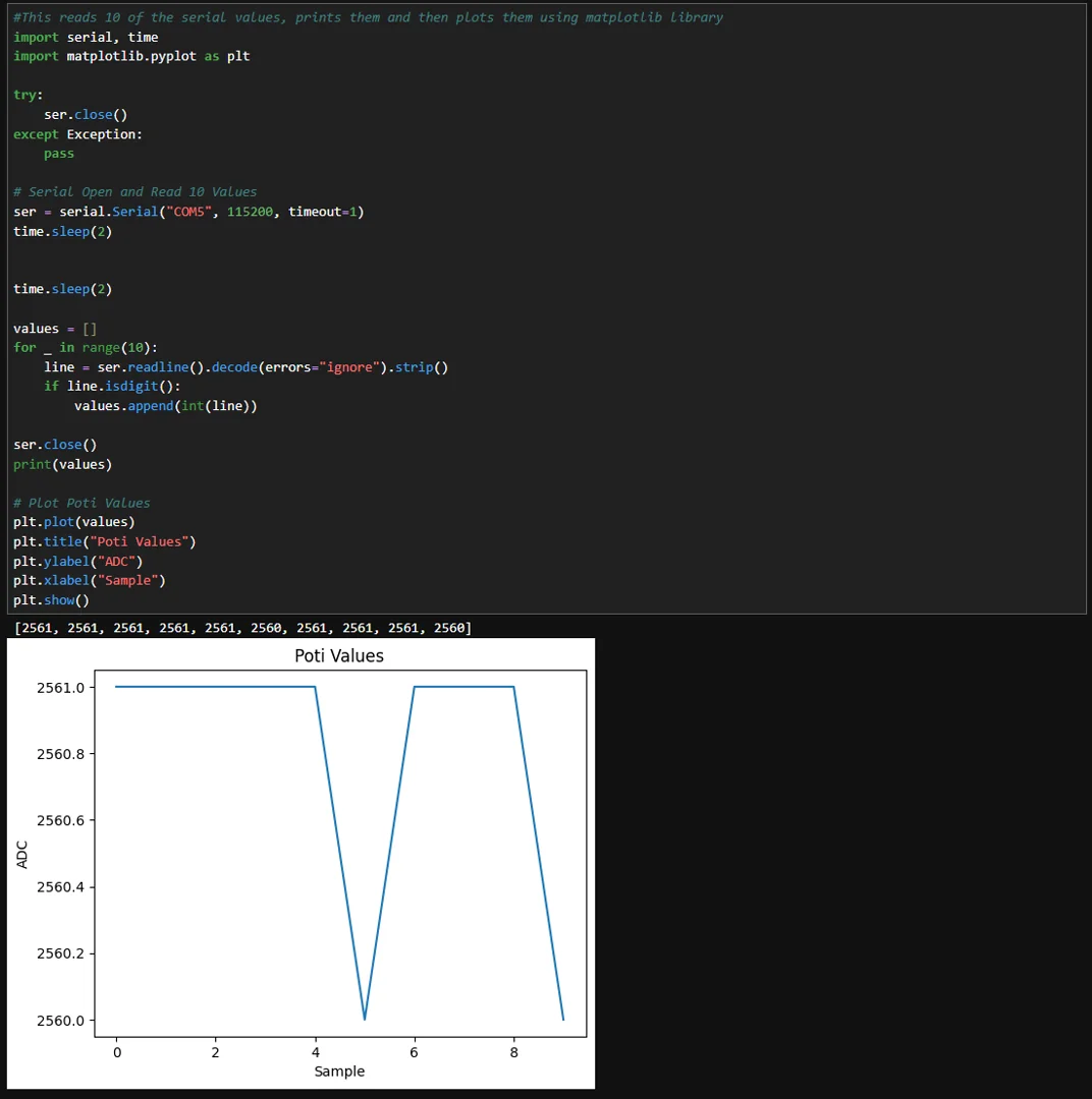
Tkinter Window with Embedded Real-Time Plot
This cell is where everything from the previous steps comes together for the first time. Rather than showing the potentiometer value as a number in a label or as a chart in a separate Matplotlib window, this script embeds a live-updating plot directly inside a Tkinter window, creating a single self-contained desktop application.
The key to making this work is FigureCanvasTkAgg, a Matplotlib backend that renders a Matplotlib figure as a Tkinter widget. Instead of calling plt.show() — which would open a separate window and block execution — the figure is attached to the Tkinter root window using canvas.get_tk_widget().pack(). From that point on, Tkinter manages the window and Matplotlib manages the chart inside it.
The update logic uses FuncAnimation, which calls an update function every 50 ms. On each call, a new value is read from the serial port and appended to a list. The Y-axis is fixed between 0 and 3168, corresponding to the observed ADC range of the ESP32. The X-axis uses a scrolling window showing the most recent 100 samples — ax.set_xlim(max(0, len(values) - 100), len(values)) — so the chart always follows the latest data rather than compressing everything into a shrinking view as more samples accumulate.
Window closing is handled cleanly via root.protocol("WM_DELETE_WINDOW", on_close), which ensures the serial port is closed before the window is destroyed. Without this, the port would remain locked after closing the window and the next cell would fail to open it.
import tkinter as tk
import serial
import matplotlib.pyplot as plt
import matplotlib.animation as animation
from matplotlib.backends.backend_tkagg import FigureCanvasTkAgg

ser = serial.Serial("COM5", 115200, timeout=0)
values = []

root = tk.Tk()
root.title("Poti Realtime Plot")

fig, ax = plt.subplots()
line, = ax.plot([], [])

canvas = FigureCanvasTkAgg(fig, master=root)
canvas.get_tk_widget().pack()

def update(frame):
    raw = ser.readline().decode(errors="ignore").strip()
    if raw.isdigit():
        values.append(int(raw))
    line.set_data(range(len(values)), values)
    ax.set_ylim(0, 3168)
    ax.set_xlim(max(0, len(values) - 100), len(values))  # scrollend
    return line,

def on_close():
    ser.close()
    root.destroy()

root.protocol("WM_DELETE_WINDOW", on_close)

ani = animation.FuncAnimation(fig, update, interval=50, cache_frame_data=False)
root.mainloop()
Real-Time ADC Noise Visualization
The companion script poti-adc-noise.py is structurally similar to the previous cell but runs as a standalone Matplotlib window without Tkinter. It uses the same FuncAnimation pattern, growing the chart in real time as new samples arrive. The difference in focus here is observational: holding the potentiometer completely still and watching the chart reveals that even a stationary input produces slightly varying ADC readings. This is normal ADC noise, and visualizing it this way makes the concept concrete and measurable in a way that a single printed number never could.
The calls to ax.relim() and ax.autoscale_view() dynamically adjust the axis scale as the data grows, so the chart always shows the full range without manual rescaling. The cache_frame_data=False setting prevents memory from growing unboundedly during long recording sessions.
import tkinter as tk
import serial
import matplotlib.pyplot as plt
import matplotlib.animation as animation
from matplotlib.backends.backend_tkagg import FigureCanvasTkAgg

ser = serial.Serial("COM5", 115200, timeout=0)
values = []
MARGIN = 20  # Y Axis around current vlaue for noise

root = tk.Tk()
root.title("Poti ADC Noise")

fig, ax = plt.subplots()
line, = ax.plot([], [])
ax.set_xlabel("Sample")
ax.set_ylabel("ADC Raw")

canvas = FigureCanvasTkAgg(fig, master=root)
canvas.get_tk_widget().pack()

def update(frame):
    raw = ser.readline().decode(errors="ignore").strip()
    if raw.isdigit():
        values.append(int(raw))

    line.set_data(range(len(values)), values)
    ax.set_xlim(max(0, len(values) - 20), max(1, len(values)))

    if values:
        center = values[-1]
        ax.set_ylim(center - MARGIN, center + MARGIN)

    return line,

def on_close():
    ser.close()
    root.destroy()

root.protocol("WM_DELETE_WINDOW", on_close)

ani = animation.FuncAnimation(fig, update, interval=50, cache_frame_data=False)
root.mainloop()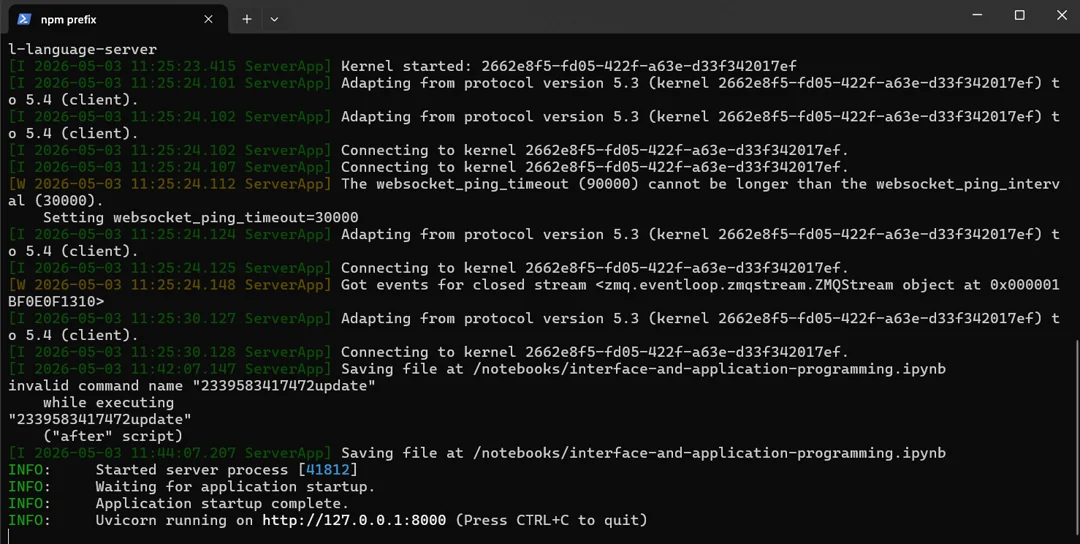
Starting the FastAPI WebSocket Server
This cell starts a local web server that bridges the serial connection and the browser. The reason this bridge is necessary is a fundamental browser security restriction: JavaScript running in a webpage cannot access the computer's serial ports directly. A local Python server acts as the middleman — it reads from the serial port and pushes the data to the browser over a WebSocket, which is a protocol designed for real-time bidirectional communication between a server and a browser.
The server is defined in server.py using FastAPI, a modern Python web framework built for async workloads. The WebSocket endpoint accepts incoming connections, then continuously reads from the serial port and forwards each valid integer value to the connected client. The server runs inside uvicorn, an ASGI server that handles the async event loop.
The runnable notebook starts uvicorn as a background process, but the code worth inspecting is the FastAPI application itself. The snippet below shows server.py: it opens the serial connection, defines the /ws WebSocket endpoint, accepts browser clients, and continuously forwards valid potentiometer values.
import serial
import asyncio
from fastapi import FastAPI, WebSocket

app = FastAPI()
ser = serial.Serial("COM5", 115200, timeout=0)

@app.websocket("/ws")
async def websocket_endpoint(ws: WebSocket):
    await ws.accept()
    ser.reset_input_buffer()  # ← Buffer leeren beim Connect
    while True:
        raw = ser.readline().decode(errors="ignore").strip()
        if raw.isdigit():
            await ws.send_text(raw)
        await asyncio.sleep(0.05)
Verifying the WebSocket Connection
This cell is a debugging step, not required for the final result. It connects to the running WebSocket server from Python itself and prints ten received values, which confirms that the server is online and data is flowing before the browser visualization is opened.
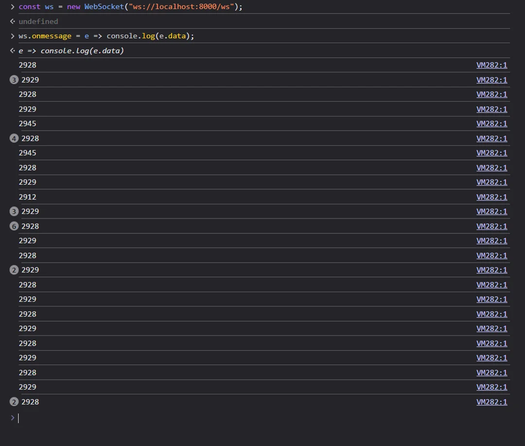
The same test can be done directly in the browser's developer console by pasting the following two lines, which is sometimes more convenient since the browser is what will ultimately consume the data:
# Check if server is up and running correctly
# This step is only for debugging because WebSocket values are otherwise invisible.
# You can also test in the browser console:
# const ws = new WebSocket("ws://localhost:8000/ws");
# ws.onmessage = e => console.log(e.data);

import asyncio
import websockets

async def test():
    async with websockets.connect("ws://localhost:8000/ws") as ws:
        for _ in range(10):
            msg = await ws.recv()
            print(msg)

await test()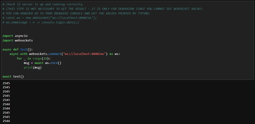
3D Visualization with three.js
This step opens poti-threejs.html in the default browser. Instead of showing only the small Python launcher, the page below shows the actual HTML and JavaScript that create the three.js scene — a 3D cube that rotates in real time as you turn the potentiometer.
The scene setup follows the standard three.js structure: a Scene object holds all the 3D elements, a PerspectiveCamera defines the viewpoint, and lights are added so the cube's material is visible. The cube itself is a simple BoxGeometry with a teal-colored standard material. The WebGL renderer is attached to the page body and sized to fill the window.
The potentiometer value arrives via the same WebSocket server started in Cell 7. A JavaScript WebSocket client listens for incoming messages and maps each raw ADC value to a rotation angle: dividing by the maximum observed value (3168) gives a 0–1 range, which is then multiplied by 2π to cover a full 360-degree rotation. This means the physical position of the potentiometer dial maps directly to the visual orientation of the cube. The current numeric value is also displayed as text on the page.
The render loop runs continuously using requestAnimationFrame, which is the browser's standard mechanism for smooth animation — it calls the render function before each screen refresh, typically at 60 frames per second.
One practical note: the current version of three.js requires an HTTP server to load as a JavaScript module, which does not work when opening a file directly from disk. For this project, an older version of three.js was used instead, which loads as a classic script tag and works with local files.
<!DOCTYPE html>
<html>
<head>
  <meta charset="UTF-8">
  <title>Poti 3D</title>
  <script src="three.min.js"></script>
  <style>
    body { margin: 0; background: #000; }
    #val { position: fixed; top: 20px; left: 20px; color: #fff; font: 32px monospace; }
  </style>
</head>
<body>

<div id="val">–</div>

<script>

const renderer = new THREE.WebGLRenderer();
renderer.setSize(window.innerWidth, window.innerHeight);
document.body.appendChild(renderer.domElement);

const scene  = new THREE.Scene();
const camera = new THREE.PerspectiveCamera(60, innerWidth / innerHeight, 0.1, 100);
camera.position.z = 4;

scene.add(new THREE.AmbientLight(0xffffff, 1));
scene.add(new THREE.DirectionalLight(0xffffff, 2));

const cube = new THREE.Mesh(
  new THREE.BoxGeometry(2, 2, 2),
  new THREE.MeshStandardMaterial({ color: 0x4f98a3 })
);
scene.add(cube);

// WebSocket
const ws = new WebSocket('ws://localhost:8000/ws');
ws.onmessage = e => {
  const v = parseInt(e.data);
  cube.rotation.y = (v / 3168) * Math.PI * 2;
  document.getElementById('val').textContent = v;
};

// Render loop
function animate() {
  requestAnimationFrame(animate);
  renderer.render(scene, camera);
}
animate();
</script>
</body>
</html>
Cleanup
Always run this cell when finished. It closes the serial connection if one is open and terminates the uvicorn server process. Skipping this step means the serial port stays locked and port 8000 stays occupied, which will cause errors the next time the notebook is run.
# close the server and the serial connection
try:
    ser.close()
except NameError:
    pass

import subprocess
subprocess.run(["taskkill", "/f", "/im", "uvicorn.exe"])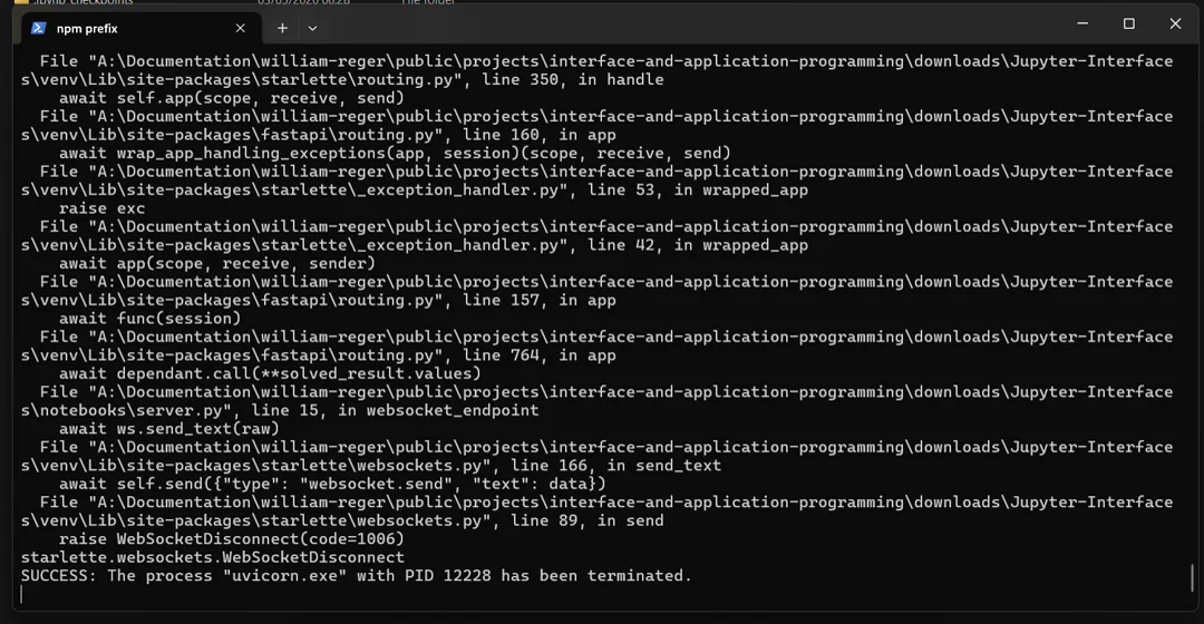

If no serial data is received, first check that the port string in the notebook matches the actual port your ESP32 is on. If you are using a Chinese Super Mini board, make sure "USB CDC on Boot" is enabled in the Arduino IDE Tools menu — without this, the board will not transmit data over USB. Unplugging and replugging the board and then restarting the kernel often resolves intermittent connection issues.
If the serial port is reported as already in use, another application — most commonly the Arduino IDE Serial Monitor — has the port open. Close it and try again.
If uvicorn fails to start with a "port already in use" error, a previous instance is still running. Run taskkill /f /im uvicorn.exe in a terminal or execute the cleanup cell first, then restart Cell 7.
If the 3D page loads but the cube does not rotate, check that the uvicorn server is running before opening the HTML file. Open the browser developer console (F12) and look for any WebSocket connection errors. If the server is not yet started, the browser will report a connection refused error.
Wireless Upgrade — MQTT
Overview
The wired setup from the notebook requires the ESP32 to be physically connected to the computer via USB. Replacing pySerial with MQTT removes that constraint entirely — the ESP32 publishes its potentiometer values over WiFi to a central message broker, the server subscribes to that topic, and everything downstream stays completely unchanged: the WebSocket, the browser, and the three.js scene are untouched.
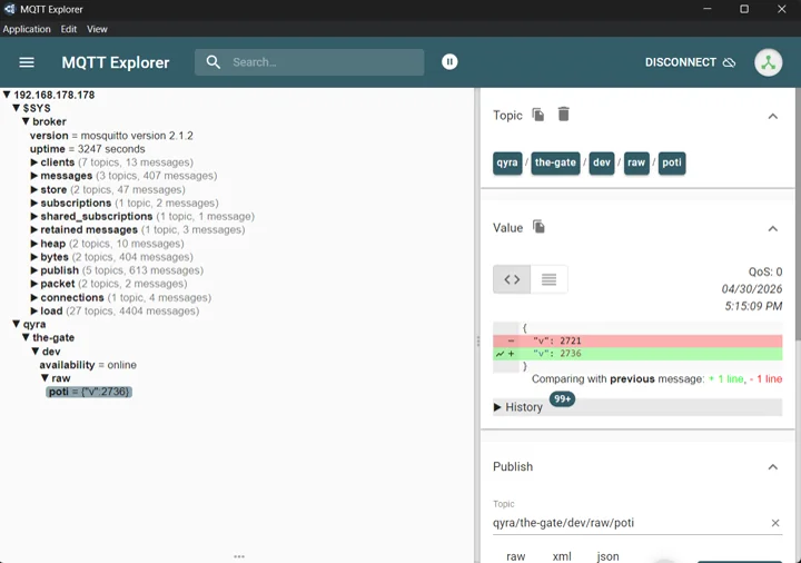
MQTT is a lightweight publish-subscribe protocol built for IoT devices. Instead of sending data directly from device to server, both sides communicate through a central broker. The ESP32 is a publisher: it connects to the broker and posts a message to a specific topic — qyra/the-gate/dev/raw/poti — whenever the potentiometer value changes meaningfully. The server is a subscriber: it tells the broker it is interested in that topic, and the broker forwards every incoming message automatically. Publisher and subscriber never communicate directly and do not need to know anything about each other, which makes the setup flexible — the hardware can sit anywhere on the network, and multiple clients can receive the same data simultaneously.
Broker Setup
The broker runs as a Docker container using Eclipse Mosquitto. Docker is a containerization platform that originated on Linux and uses kernel features to run isolated processes — think of a container as a lightweight, self-contained package that includes an application and everything it needs to run, without the overhead of a full virtual machine. It runs on any Linux server, Raspberry Pi, or NAS, and is the standard way to self-host small services like this. Getting Mosquitto running takes a single line — no config file required for a basic local setup:
This starts the broker in the background, exposes port 1883 on the host machine, and allows unauthenticated connections from the local network. The ESP32 firmware then connects to the host IP, applies a deadband of 8 ADC units and a minimum send interval of 50 ms to filter out noise, and publishes {"v":n} on each meaningful change. On the server side, pySerial is simply replaced by a paho-mqtt subscription to the same topic — the value arrives identically and is forwarded through the existing WebSocket pipeline to the browser.
docker run -d --name mosquitto -p 1883:1883 eclipse-mosquitto \
  sh -c "echo 'listener 1883\nallow_anonymous true' > /mosquitto/config/mosquitto.conf && mosquitto -c /mosquitto/config/mosquitto.conf"
MQTT Explorer Debugging
For debugging, MQTT Explorer is the go-to tool. It is a desktop application that connects directly to the broker and displays all active topics in a hierarchical tree view, showing incoming messages in real time with their full payload. You can see exactly what the ESP32 is publishing, inspect the JSON payload, check timestamps, and even publish test messages manually — which means you can drive the three.js visualization without any hardware at all, just by typing a value into MQTT Explorer and hitting send.