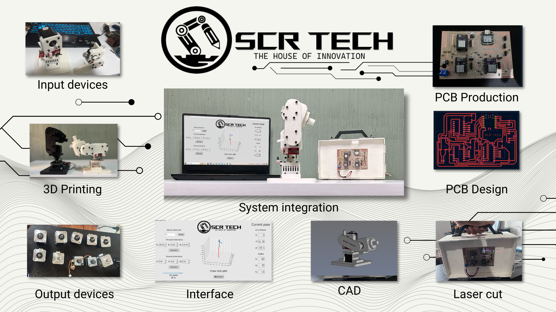
FINAL PROJECT 3 DOF Open source robotic arm
To facilitate the reader's navigation through the activities carried out for this project, I am attaching the list of activities.
- Cycloidal drive design
- Cycloidal drive manufacturing
- Cycloidal drive testing
- Electronic board design
- Electronic board manufacturing
- Electronic board testing
- Electronics box design and manufacturing
- Software development
- System integration
- Robot files
This project was full of difficulties in its development. For the reader, I have attached a slide with its main characteristics, as well as a presentation video and the entire process to develop this first prototype. I hope you enjoy it.
Cycloidal drive design
The development of a cycloidal reducer involved many phases in the development process since it is the cornerstone of the mechanism. The movement of the system depends on these small modules. For this project, I developed more than four prototypes, one of them for the Nema 23 and the final prototype for the Nema 17. I will start by describing the procedure for its design.
The heart of a cycloidal reducer is the cycloidal disk that resides inside it. There are many and varied ways to design this piece; however, in all cases, its geometry depends on the following equations:
- x = R*cos(theta) - Rr*cos(theta - phi) - E*cos(N*theta)
- y = -R*sin(theta) + Rr*sin(theta - phi) + E*sin(N*theta)
- phi = -arctan((sin((1-N)*theta))/((R/(E*N))-cos((1-N)*theta)) t.q. 0 <= theta <= 2pi
However, due to the design tool I used for the development of this project (SolidWorks), it is completely necessary to use the parametric form of these equations, which are as follows:
- X = (R*cos(t))-(Rr*cos(t+arctan(sin((1-N)*t)/((R/EN)-cos((1-N)*t)))))-(E*cos(N*t))
- Y = (-R*sin(t))+(Rr*sin(t+arctan(sin((1-N)*t)/((R/EN)-cos((1-N)*t)))))+(E*sin(N*t))
- T1 = (-10/360) * 2*pi
- T2 = (190/360) * 2*pi
Where:
- R is the radius of the rotor
- E is the eccentricity of the cycloidal disk
- Rr is the radius of the rollers
- N is the number of rollers of the estator
The idea behind designing a cycloidal reducer is to play with these parameters until you obtain a disk that meets the desired reduction ratio and makes sense with the existence of mechanical parts such as bearings and screws. The optimization process took me several prototypes. To achieve this, I created the following Python script, which helps ensure that the curve generated by the parametric equations does not intersect, meets the reduction ratio I am looking for, and also prints the parametric equations in a format understandable by SolidWorks. This script significantly speeds up the workflow.
                    import numpy as np
                    import matplotlib.pyplot as plt

                    #Cycloidal disk parameters
                    R = 30.7
                    E = 0.5       # E < R/N
                    Rr = 1.5
                    N = 48

                    #Parametric equations definition
                    t = np.linspace(0, 2*np.pi, 1000)
                    X = R * np.cos(t) - Rr * np.cos(t + np.arctan(np.sin((1-N)*t) / (R/(E*N) - np.cos((1-N)*t)))) - E * np.cos(N*t)
                    Y = -R * np.sin(t) + Rr * np.sin(t + np.arctan(np.sin((1-N)*t) / (R/(E*N) - np.cos((1-N)*t)))) + E * np.sin(N*t)

                    #Convert the format
                    t_symbol = "t"
                    cos_t = f"cos({t_symbol})"
                    sin_t = f"sin({t_symbol})"
                    cos_Nt = f"cos({N}*{t_symbol})"
                    sin_Nt = f"sin({N}*{t_symbol})"
                    cos_1Nt = f"cos((1-{N})*{t_symbol})"
                    sin_1Nt = f"sin((1-{N})*{t_symbol})"
                    atan_expr = f"arctan({sin_1Nt}/(({R}/({E}*{N}))-{cos_1Nt}))"

                    X_eq = f"({R}*{cos_t})-({Rr}*cos({t_symbol}+{atan_expr}))-({E}*{cos_Nt})"
                    Y_eq = f"(-{R}*{sin_t})+({Rr}*sin({t_symbol}+{atan_expr}))+({E}*{sin_Nt})"

                    print("Parametric equations for SolidWorks input:")
                    print(f"X = {X_eq}")
                    print(f"Y = {Y_eq}")

                    #Graph the equations
                    plt.figure(figsize=(8, 8))
                    plt.plot(X, Y, label='Cycloidal disk contour')
                    plt.title('Cycloidal disk graph')
                    plt.xlabel('X')
                    plt.ylabel('Y')
                    plt.axis('equal')
                    plt.legend()
                    plt.grid(True)
                    plt.show()
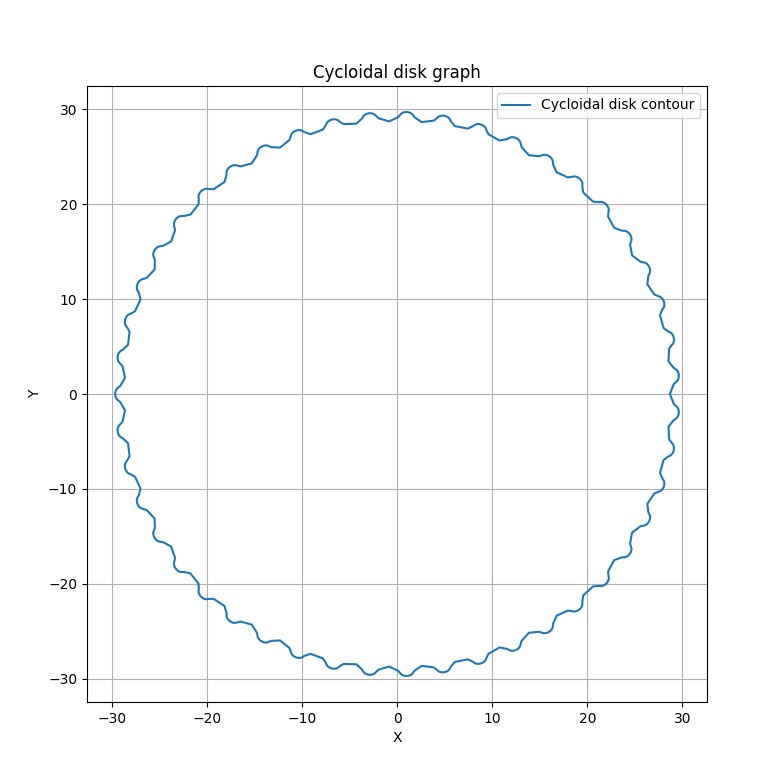
The following image shows the graph generated by matplotlib for the parameters I entered. It should be noted that this cycloidal disk is designed for a 48:1 reduction, and the equations obtained are those I used for the final cycloidal disks of my project. This script greatly facilitated the process of finding the appropriate tolerances for 3D printing, as it allows modifying the disk radius and thus enables testing with a single stator.
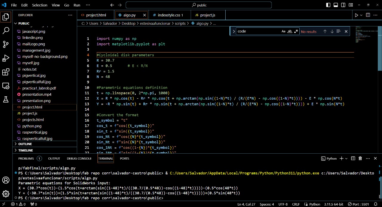
The following image shows the console output, we will use them later once we are in SolidWorks.
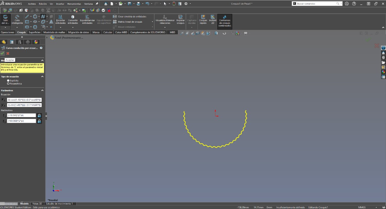
At this point, we can begin with the design. Once we are in SolidWorks, we go to the 'Tools' tab, and in the 'Sketch Entity' section, we select the option for 'Equation Driven Curve'.

The following menu will appear. In the 'Equation Type' section, we will select 'Parametric' and enter the equations prepared by Python, as well as the values of t1 and t2 that I mentioned in the mathematical definition of the curve. The following geometry will then be displayed.
Next, we will draw a construction line along the x-axis of the Cartesian plane to trim the excess entities, and then evenly distribute the resulting entity along the same construction line. Afterward, we will extrude the design, and it will look as follows.

This is the most interesting part of the design, for which many considerations must be taken into account. The rest of the design can be inferred, so I will proceed to show the result of the reducer that I used in my project, already assembled.

The following video shows a brief motion simulation to ensure that the design is mathematically coherent. During the manufacturing stage, I faced the challenge of finding the correct tolerances. The simulation is shown below.
Cycloidal drive manufacturing
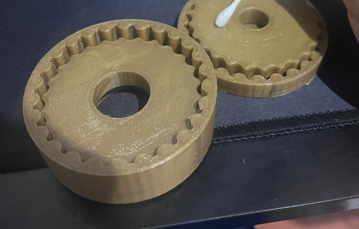
As I mentioned, the manufacturing of the cycloidal reducer was a stage of too many iterations. I first designed the system to understand its functioning and verify that the parts fit together. The following photograph shows the first version I made of the reducer.
Once I verified the operation of the cycloidal disk, I proceeded to take a step further and redesign everything to be able to couple it to the Nema 23 motor that I was planning to use at the beginning of the project.

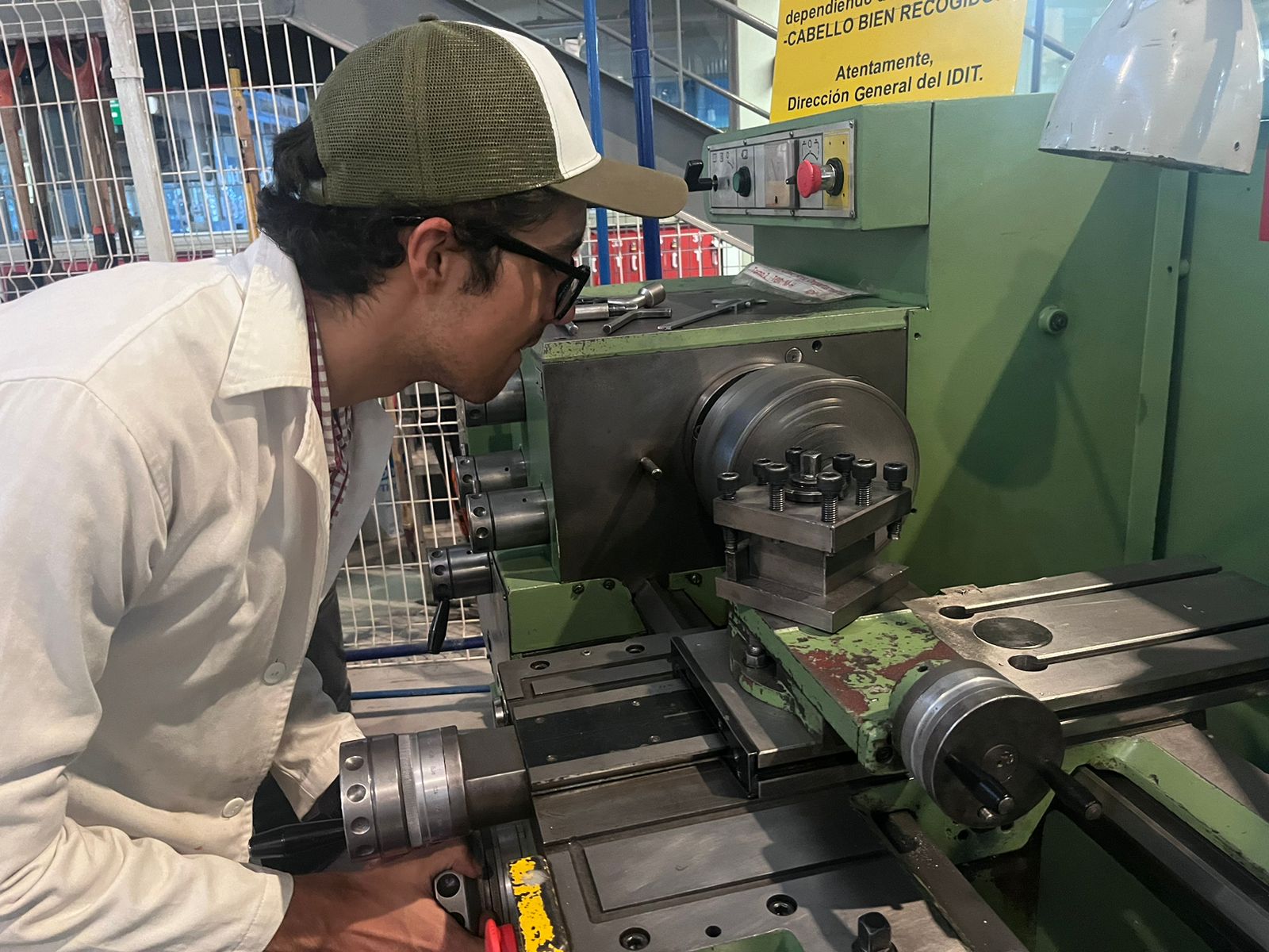
Then I hypothesized that I would need some aluminum parts inside the reducer to make it more robust, so I got an 8mm thick aluminum tube. Due to the tolerances in the printing, I had to machine the tube on the lathe.
This is what the reducer looked like after I installed the aluminum tubes machined on the lathe.
After designing a cover for this version of the reducer, things started to take shape, and it looked like this on the Nema 23.
At this point, it was time to conduct the first tests. The following video shows the reducer in operation; it generated too much vibration, and that's why I decided to use more compact and sealed reducers for the Nema 17. However, the test of the operation of this 25:1 reducer manufactured for the Nema 23 is shown next.
At this point, I was convinced to continue down this path. Attached below is the latest version of the 25:1 reducer manufactured for the Nema 23.
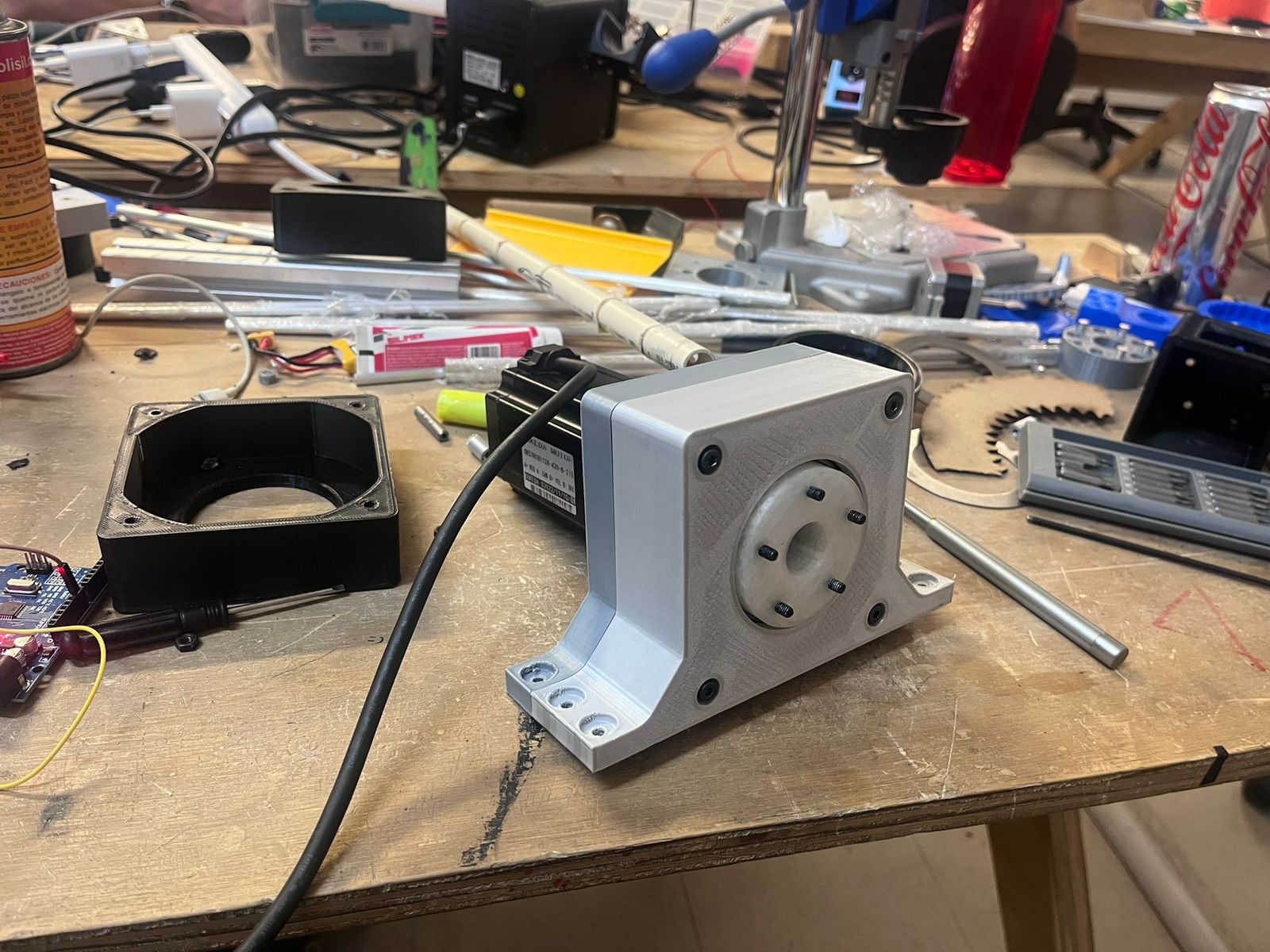
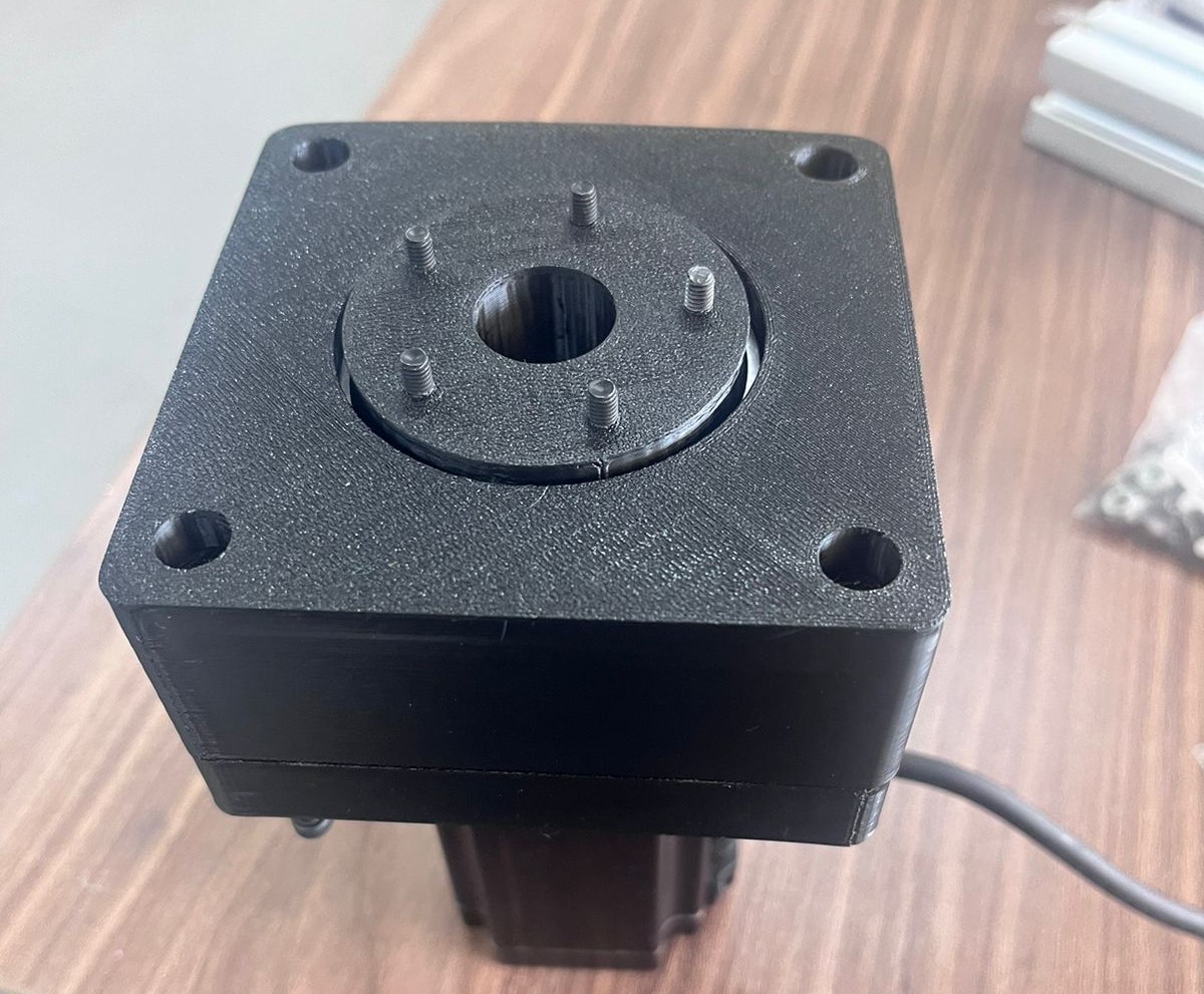
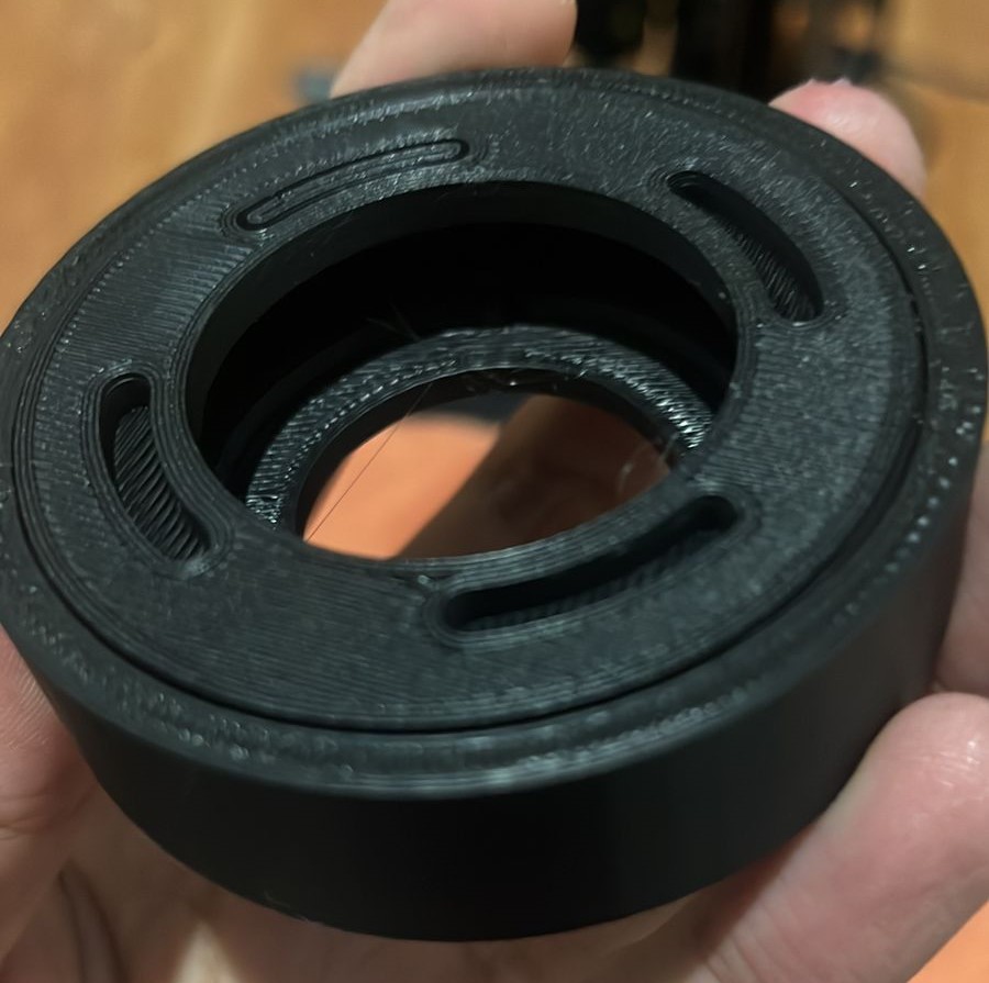
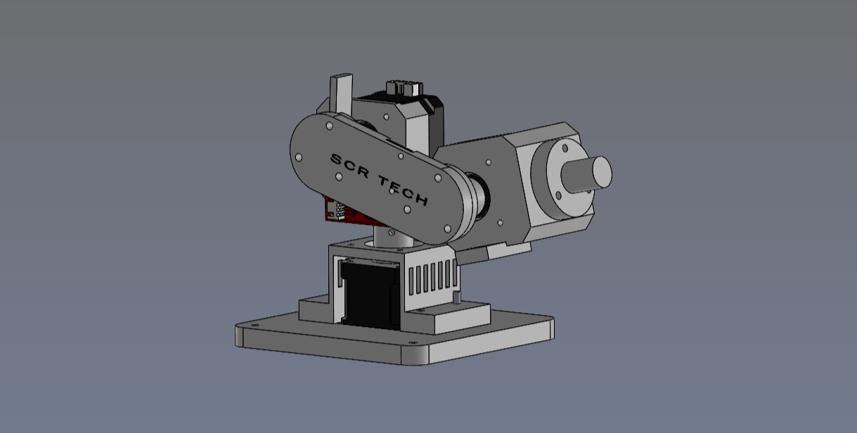
After redesigning several things and conducting extensive internet research, I decided to use the knowledge I had already acquired along with a cycloidal prototype I found online to create a more compact and sealed 48:1 reducer version for the Nema 17. The following image shows the final assembled version of the reducer.
Cycloidal drive testing
As I mentioned, I conducted numerous tests to observe, verify, and improve the functioning of the cycloidal reducer. The following video shows one of the many versions I adapted for the Nema 23 operating without the extractor. It's mesmerizing to watch the cycloidal disk performing its general plane movement.
Since the amount of information I have from the tests conducted is greater than the amount of free time I have lately, in this section, I will only attach one more video, showing the first version of the final reducer in operation.
Electronic board design
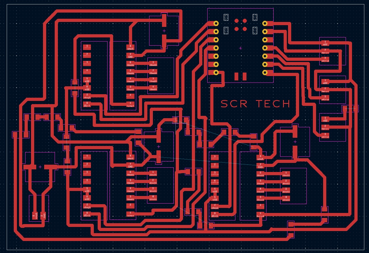
For the electronic design part, I decided to use the KiCad software for a very simple reason: from the first design session, I installed a library of components available in my fablab. Although sometimes the component isn't available, it is an excellent starting guide for designing without complications. The final board design is shown below.
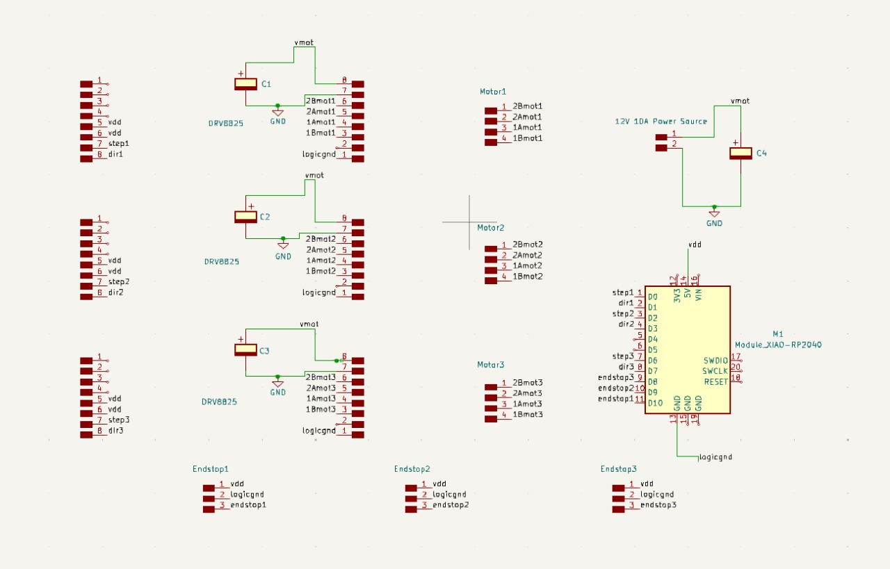
The circuit schematic is shown below. It is worth noting that the 19 ghost resistors I used for the board tracks are not present in the schematic to allow for a clear view of the connections. There are some unusual practices in the schematic, such as calling the microcontroller ground "logicgnd." I did this because I am using female headers to create a socket for each module, and the DRV8825 already has that connection internally.
Electronic board manufacturing
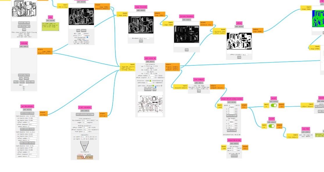
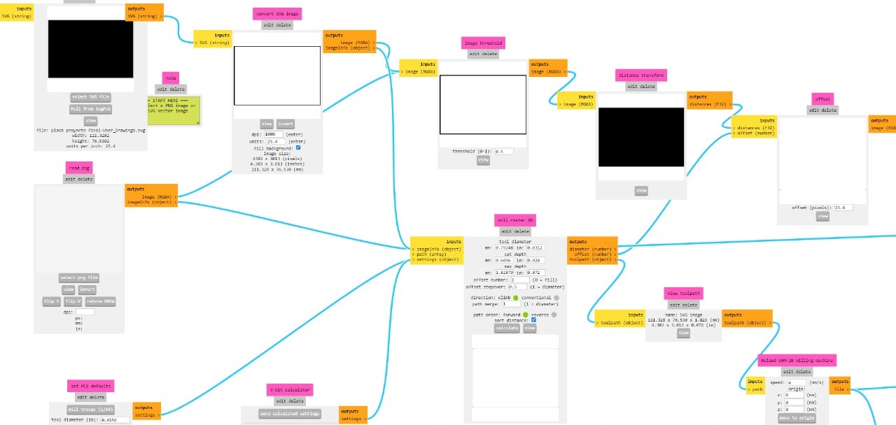
For the manufacturing stage, the first task was to generate the G-code for engraving and cutting the board. I used the parameters that I have been using throughout the weeks to generate the G-code. Below is an image of mods to generate the engraving G-code.
And the following image shows the parameters used fot the cutting stage.
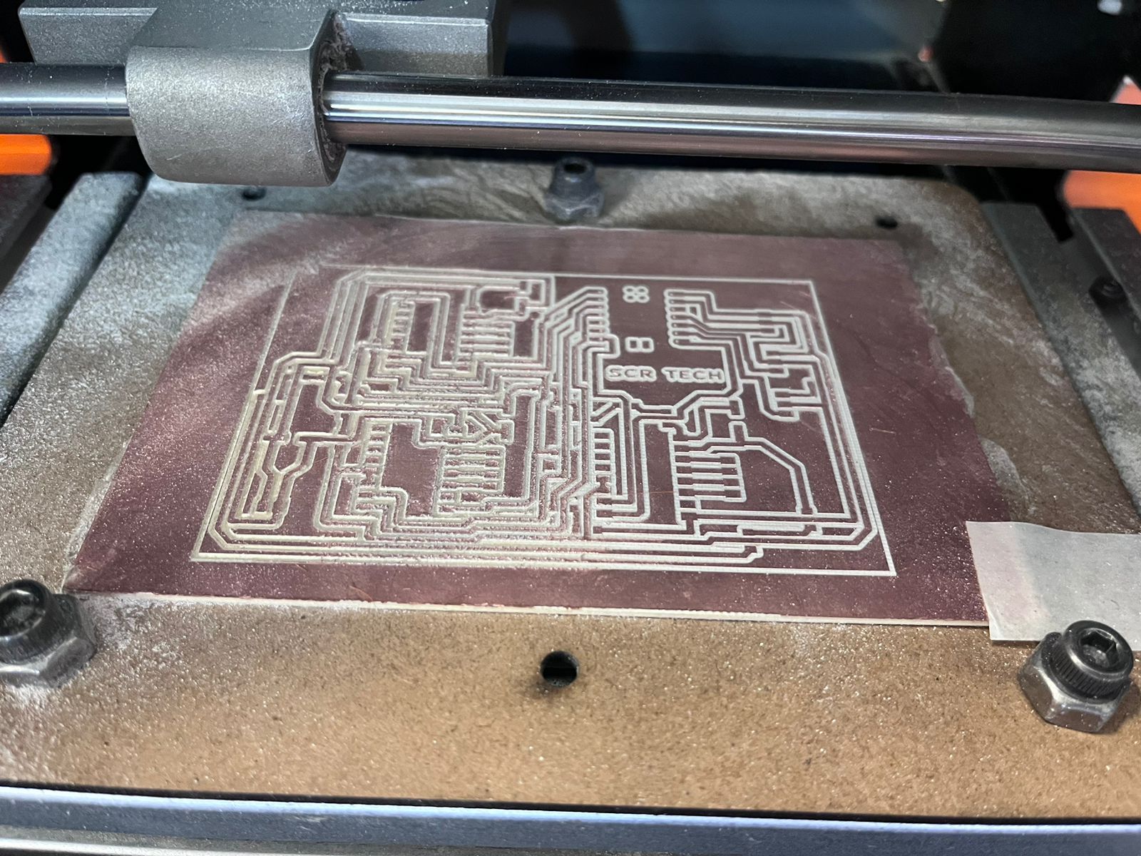
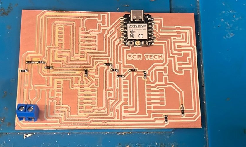
Once I had the G-code for the two manufacturing stages, I decided to take precautions and level the bed of the Roland Mini Mill. This was because the dimensions of the board are considerable (approximately 12cm x 8cm). When I confirmed the proper leveling of the bed, I simply began the manufacturing process, which was somewhat lengthy (approximately 3 and a half hours). The following image shows the board just after the engraving process.
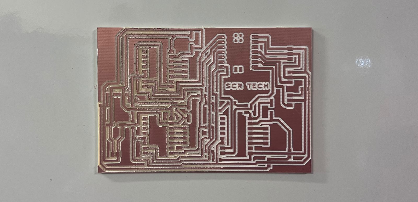
After the engraving and cutting process, I simply extracted the board carefully. The board, freshly removed from the sacrificial bed, looks like the one in the following image.
Having reached this point, it was time to solder, so I went to my Fablab soldering station where I soldered the components of the board. I started by soldering the 19 phantom resistors, the terminal block of the power stage, and the Xiao ESP32 - C3.
Then I soldered the female pins of each DRV8825, followed by the decoupling capacitors. Several hours passed soldering, and in the end, the board looked like this.
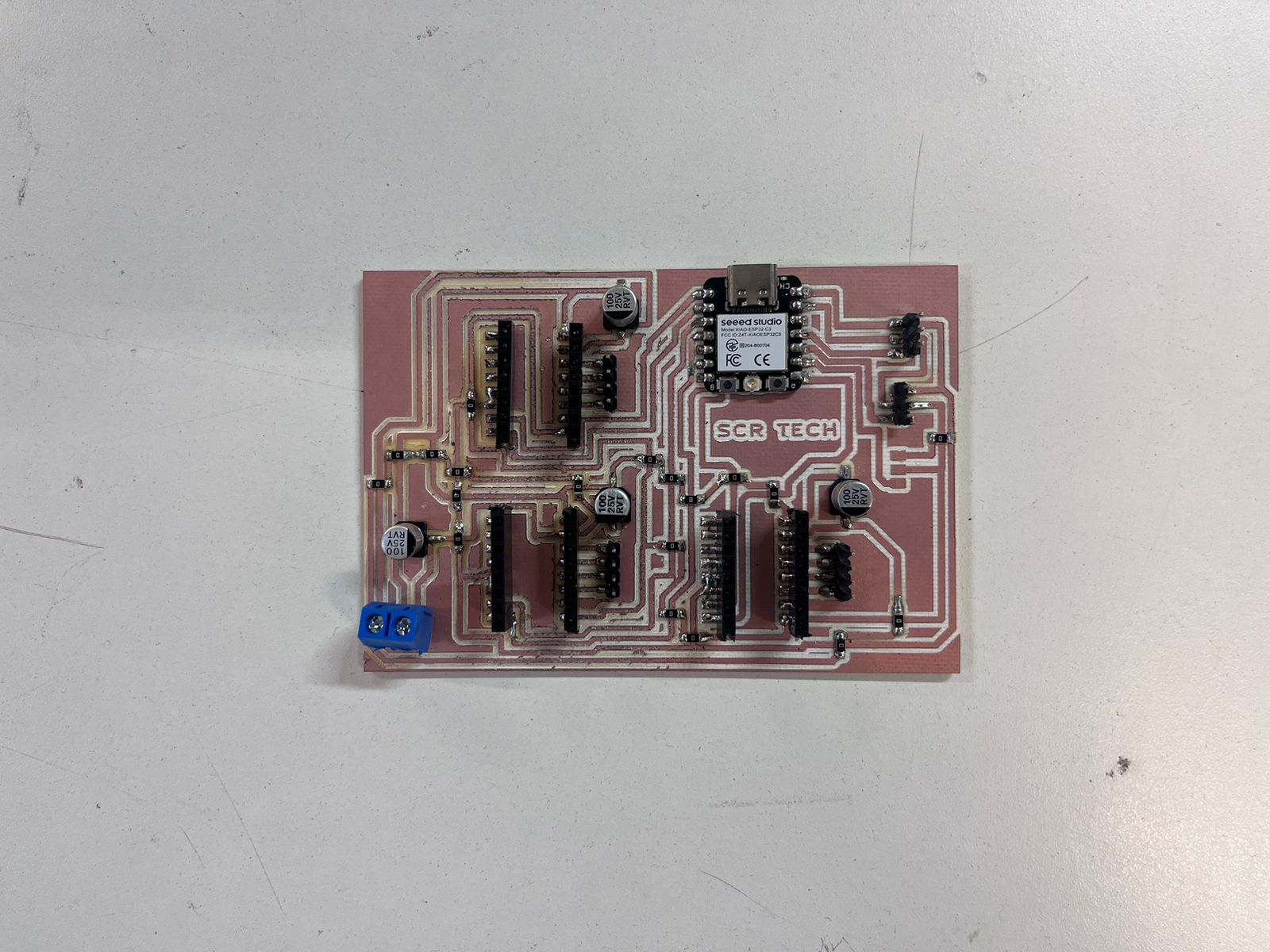
In the previous image, you can see that 3 male pins are missing. This is because
the pins ran out at my FabLab, so when I got home, I soldered the remaining pins.
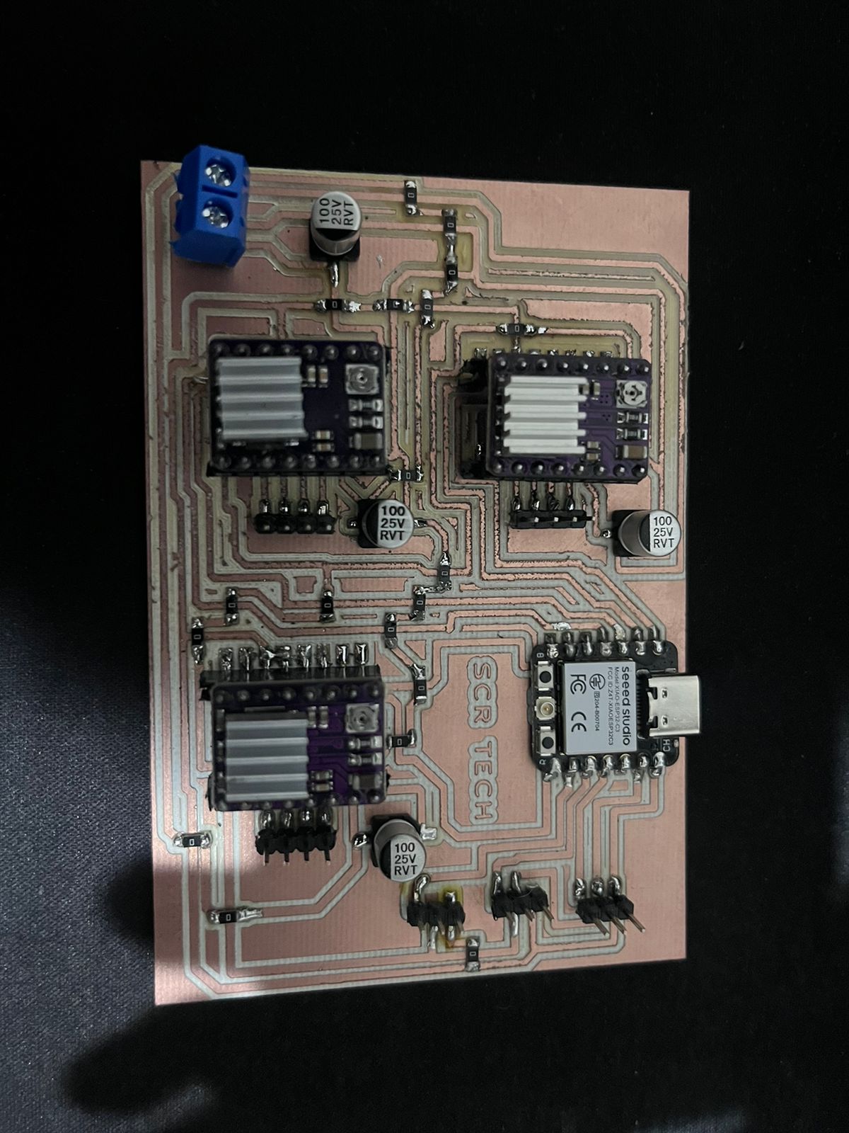
I attached a heatsink to each DRV8825, placed the drivers in their positions, and
adjusted their maximum current to 1.4A since my motors are rated at 1.8A. The following
image shows the board with all its components in place.
Electronic board testing
To check the operation of my system, I wrote the following script:
                    //Each motor's Pin and Dir
                    #define STEP_PIN 2
                    #define DIR_PIN 3
                    #define STEP_PIN_2 4
                    #define DIR_PIN_2 5
                    #define STEP_PIN_3 21
                    #define DIR_PIN_3 20

                    //Endstops
                    #define Endstop1 10
                    #define Endstop2 9
                    #define Endstop3 8

                    void setup() {
                      //Motor 1
                      pinMode(STEP_PIN, OUTPUT);
                      pinMode(DIR_PIN, OUTPUT);

                      //Motor2
                      pinMode(STEP_PIN_2, OUTPUT);
                      pinMode(DIR_PIN_2, OUTPUT);

                      //Motor3
                      pinMode(STEP_PIN_3, OUTPUT);
                      pinMode(DIR_PIN_3, OUTPUT);

                      // Configure endstop pins as input with pull-up
                      pinMode(Endstop1, INPUT_PULLUP);
                      pinMode(Endstop2, INPUT_PULLUP);
                      pinMode(Endstop3, INPUT_PULLUP);

                      //Start serial communication to print values
                      Serial.begin(9600);
                    }

                    void loop() {
                      //Read state of the endstop switches
                      int switchState1 = digitalRead(Endstop1);
                      int switchState2 = digitalRead(Endstop2);
                      int switchState3 = digitalRead(Endstop3);

                      //Print states of the switches
                      Serial.print("Endstop1: ");
                      Serial.println(switchState1);
                      Serial.print("Endstop2: ");
                      Serial.println(switchState2);
                      Serial.print("Endstop3: ");
                      Serial.println(switchState3);

                      //Move motor 1 in one direction
                      digitalWrite(DIR_PIN, HIGH);

                      //Generate pulses to move motor 1
                      for (int i = 0; i < 200; i++) {  //200 steps per revolution for a 1.8 degree per step motor
                        digitalWrite(STEP_PIN, HIGH);
                        digitalWrite(STEP_PIN_2, HIGH);
                        digitalWrite(STEP_PIN_3, HIGH);
                        delayMicroseconds(500);  //Adjust according to the desired speed
                        digitalWrite(STEP_PIN, LOW);
                        digitalWrite(STEP_PIN_2, LOW);
                        digitalWrite(STEP_PIN_3, LOW);
                        delayMicroseconds(500);  //Adjust according to the desired speed
                      }

                      delay(1000);  //Wait before reversing direction

                      //Move motor 1 in the opposite direction
                      digitalWrite(DIR_PIN, LOW);

                      //Generate pulses to move motor 1 in the opposite direction
                      for (int i = 0; i < 200; i++) {
                        digitalWrite(STEP_PIN, HIGH);
                        digitalWrite(STEP_PIN_2, HIGH);
                        digitalWrite(STEP_PIN_3, HIGH);
                        delayMicroseconds(500);  //Adjust according to the desired speed
                        digitalWrite(STEP_PIN, LOW);
                        digitalWrite(STEP_PIN_2, LOW);
                        digitalWrite(STEP_PIN_3, LOW);
                        delayMicroseconds(500);  //Adjust according to the desired speed
                      }

                      delay(1000);  //Wait before moving again in the original direction
                    }
Subsequently, I made the relevant connections between: motors, end switches, and the 12V 10A switched power supply.
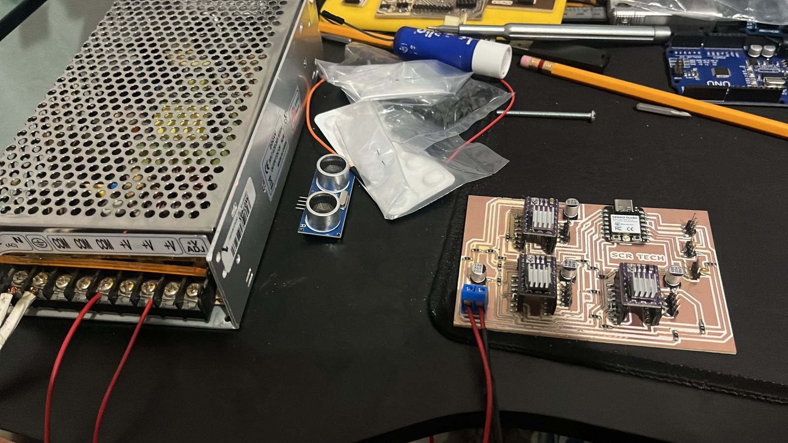
And the moment of truth had arrived, the following video shows the correct functioning of the board to control the 3 stepper motors and the 3 limit switches.
Electronics box design and manufacturing
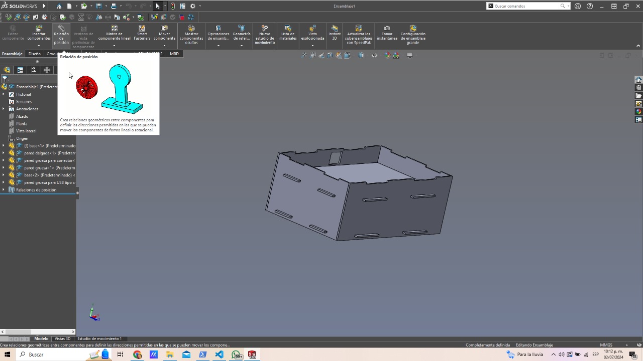
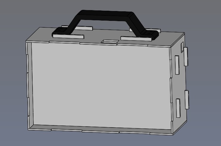
For the design of the box that hides the power and control stage from the user, I simply designed a portable box. The following image shows the design of the box.
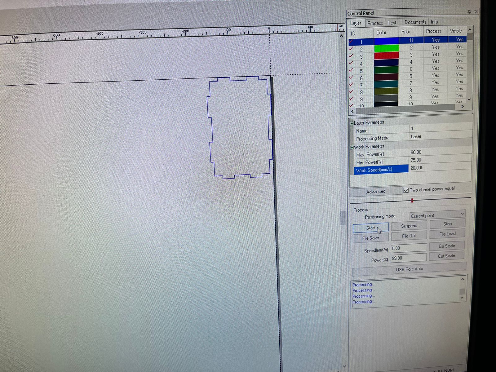
Then I went to the laser cutting machine and first cut acrylic and then MDF, the following image shows the parameters i have used for the acrylic cut.
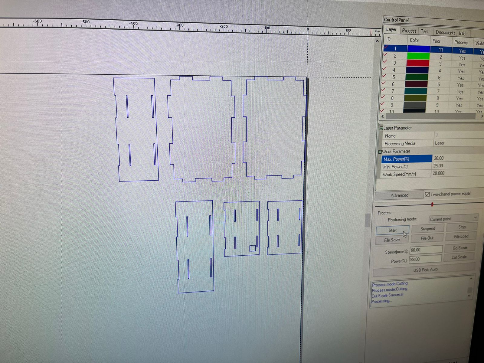
Subsequently, cut the MDF with the following parameters.
This is how my MDF board looked after the laser cutting.

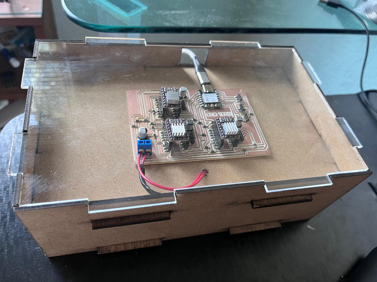
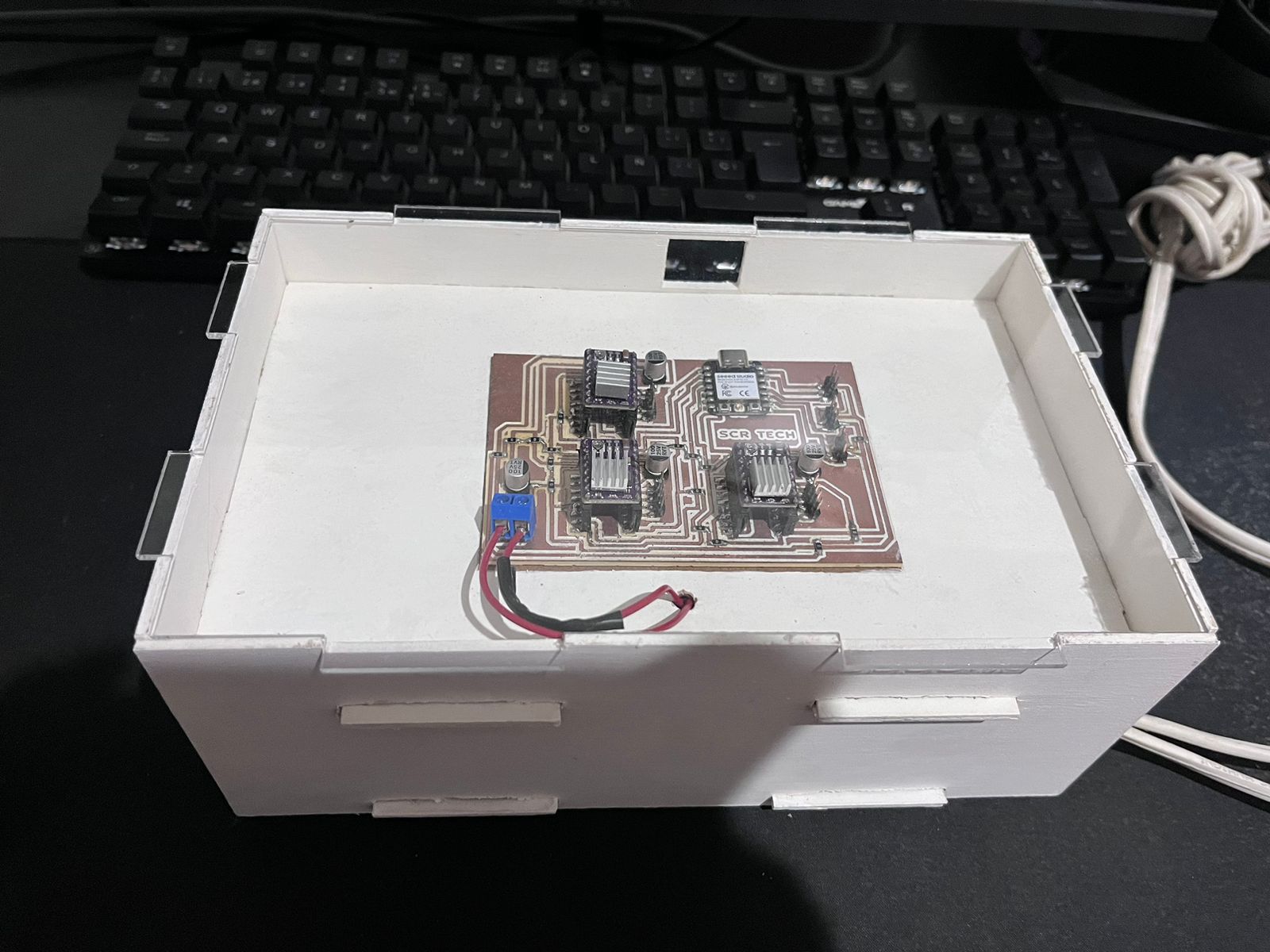
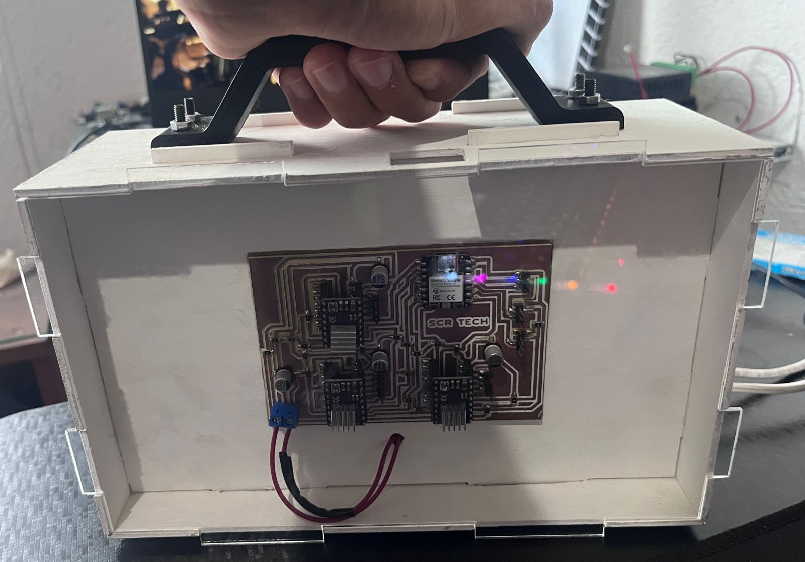
The following image shows the final electronic box already manufactured.
When I saw the box, I felt it lacked a bit of style, so I spent an afternoon painting the entire box white.
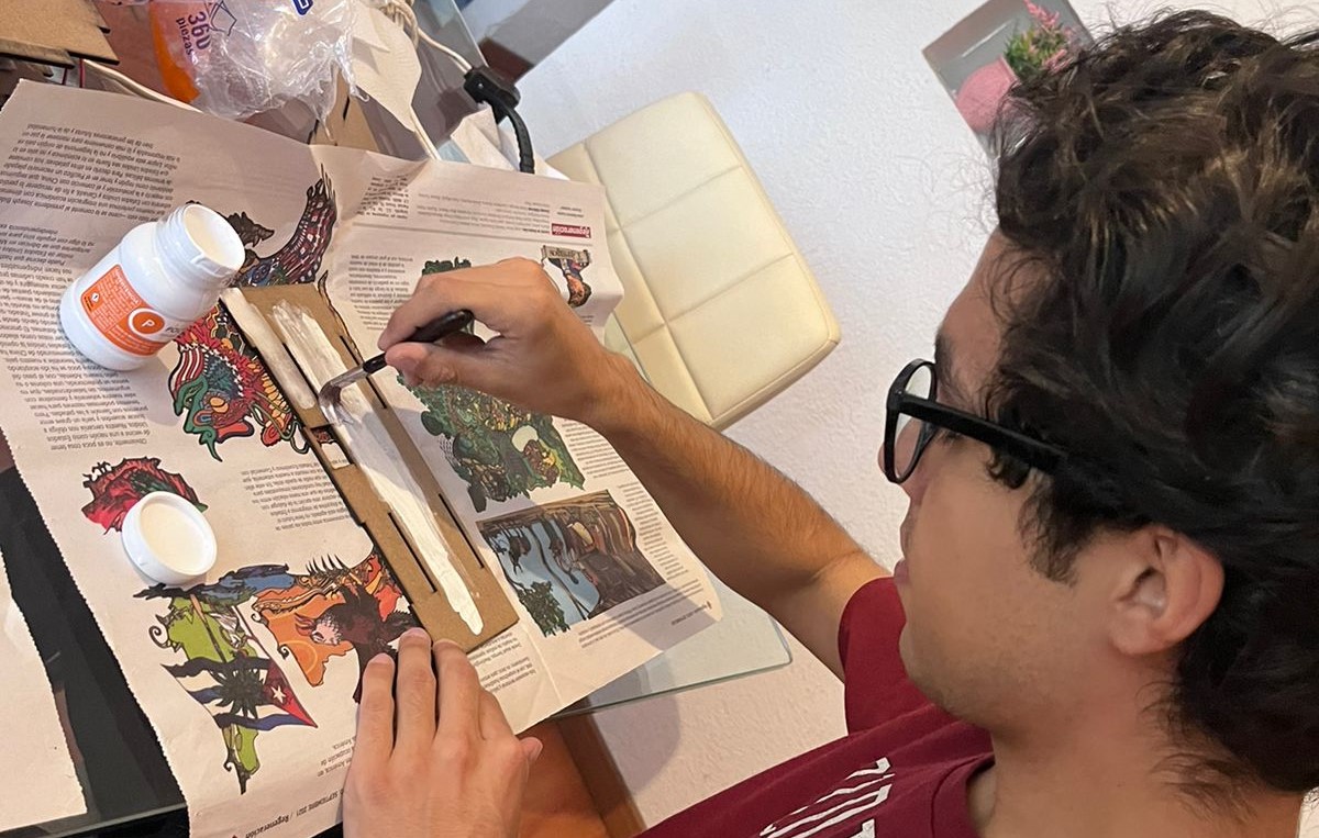
As soon as I finished painting the box and reassembling the pieces, the final result looked much more aesthetic. Below, I show the painted and assembled box.
As soon as the box was assembled, I came up with the idea of designing a handle to improve the user experience. Below, I show the 3D model.
I proceeded to print the handle; the following image shows the handle freshly out of the printer.

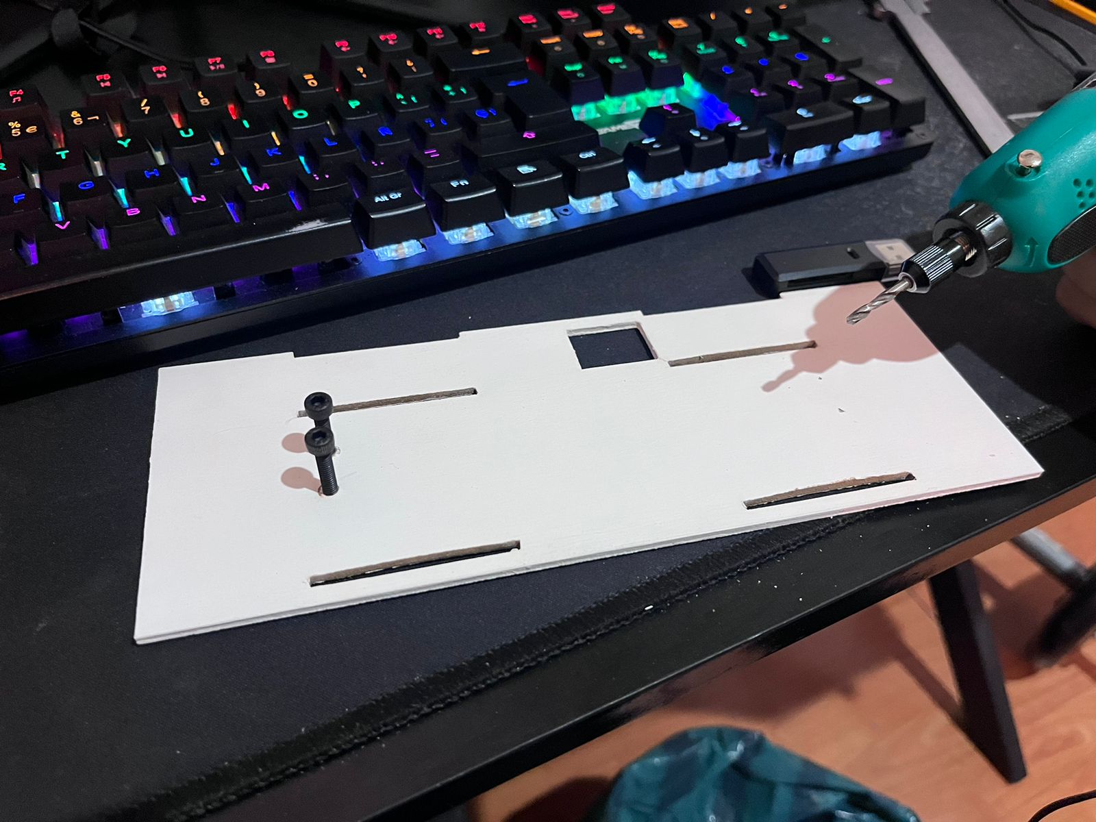
Then I made some holes with the Dremel in the part of the box where I decided to place the handle.
The final result is shown below.
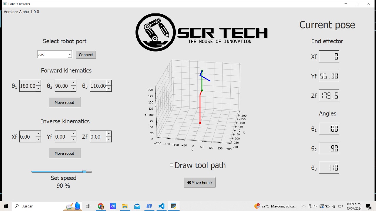
Software development
To successfully control the robot, I had to perform several tests to determine the range of speeds the system can achieve. Fortunately, I found that the robot can move between 30 and 60 steps/sec without any issues. Additionally, I calculated both the forward and inverse kinematics myself. I spent a lot of time working with the kinematic simulation I created in Matplotlib, which can now be seen in the center of the interface. To view the detailed development of the interface, you can click here.
System integration
Unfortunately, the performance of all the reducers I developed for this project was severely compromised by vibrations, making the system very strong but not precise. Therefore, to showcase the entire mathematical and software development I did for this project, I opted for a simplified, smaller, and more precise robot model with stepper motors directly coupled to each joint.
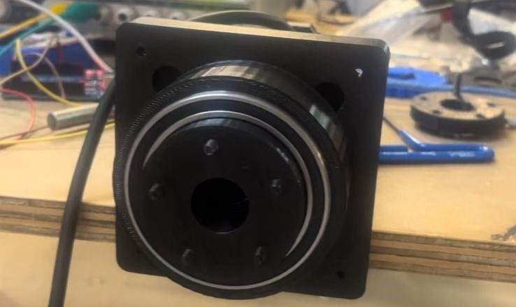
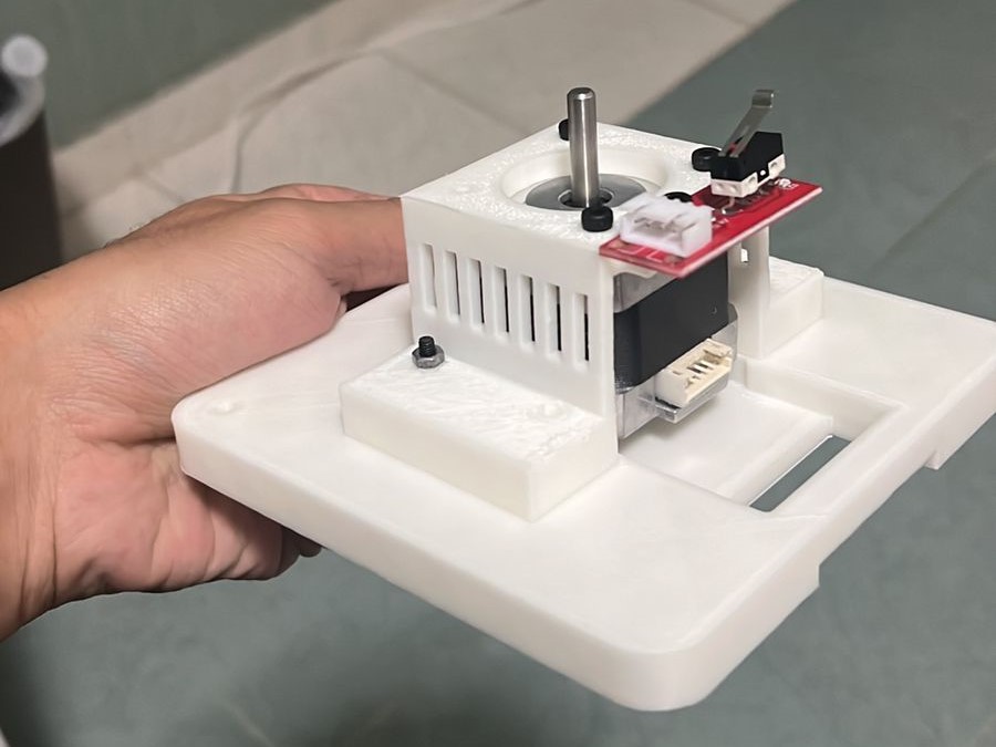
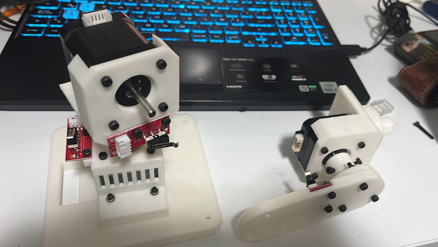
After verifying the design's functionality in SolidWorks, I started manufacturing the system's parts and gradually began assembling the robot. I started with the base. The following image shows the first joint with its own limit switch.
After a while assembling everything, all that was left was to print one last coupling to put the whole system together.
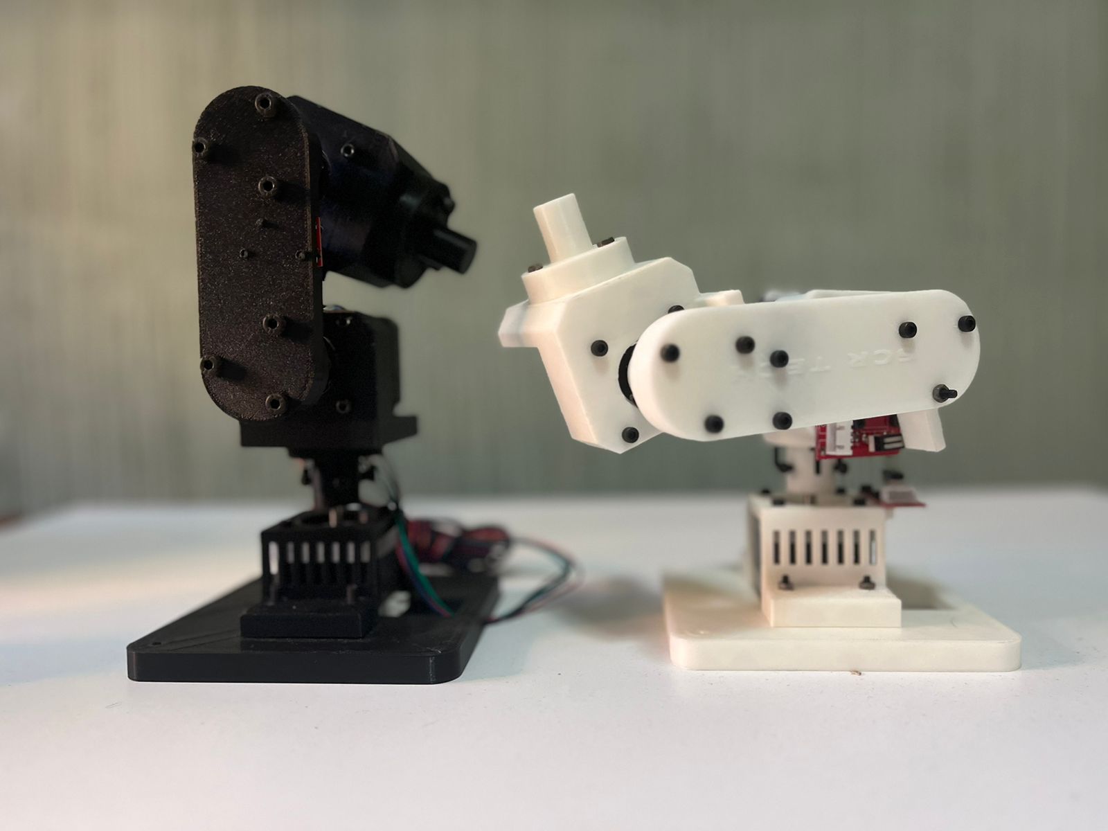
Finally, I finished assembling the system, and the result was amazing. I decided to take the following photo with the first prototype of the robot.
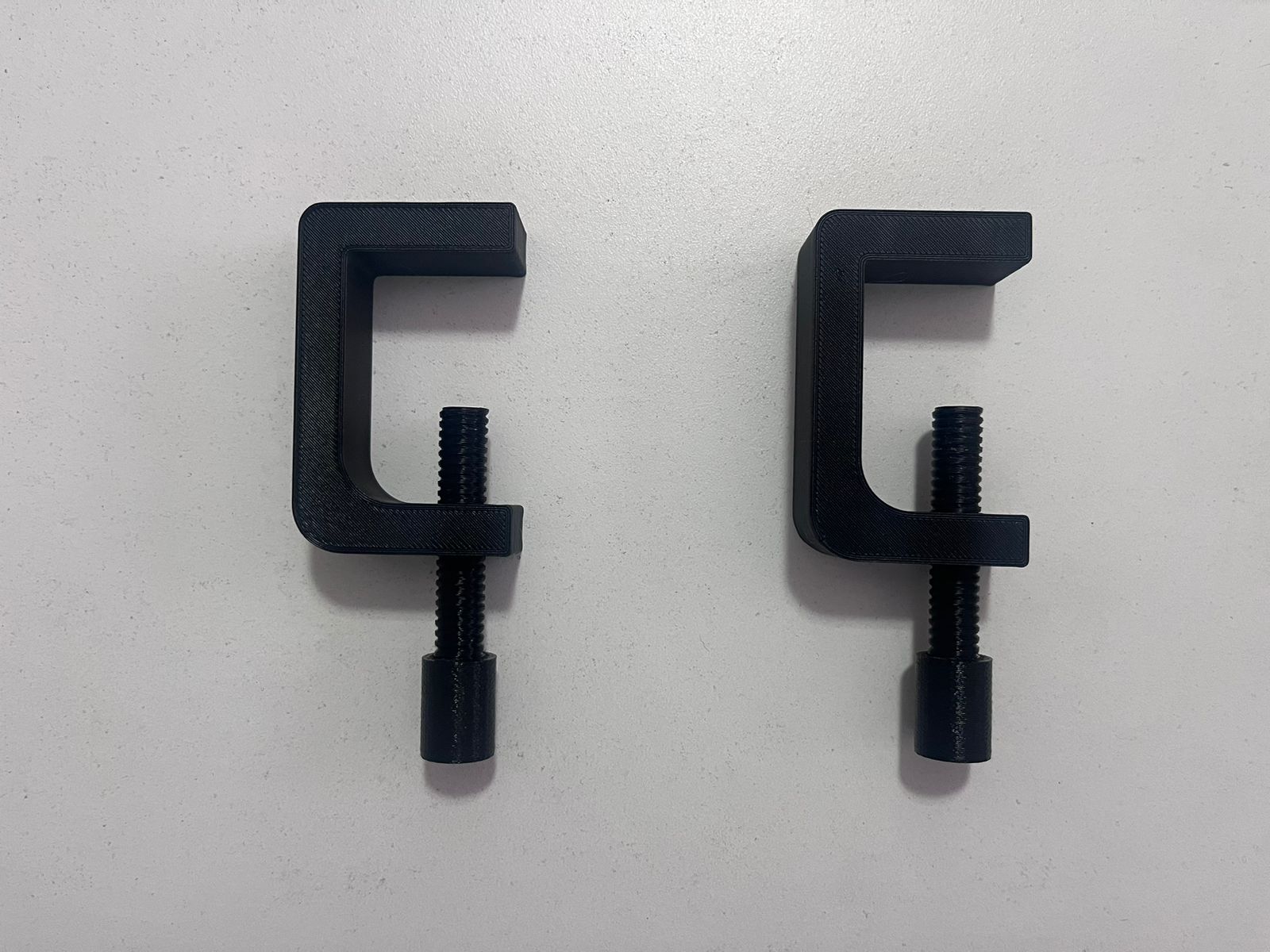
After conducting some tests, as the reader can see in the video at the end of the system integration section, the robot vibrates a lot, causing the base to move. Therefore, I designed and manufactured the following clamps.
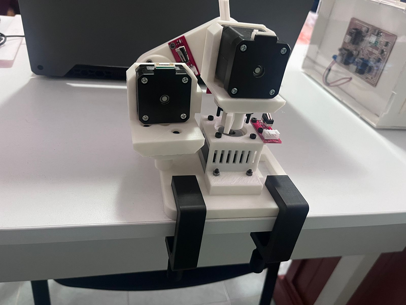
To secure the structure, it is as simple as using the clamps between the table and the robot, as shown in the following image.
Finally, to demonstrate the operation of each component of the system, I have attached the following video where I also give a brief explanation of how to use the robot.
Robot files
Below, I have attached all the files to manufacture and use the robot.
Final thoughts
The process of designing, manufacturing, and integrating systems for a robotic arm is a complex process that involves a preliminary planning stage and a long period of experimentation, especially in the manufacturing stage. Personally, I joined FabAcademy because I am generally good at solving the theoretical aspects of a project; however, manufacturing has never been my strong suit. After all the time invested, I am satisfied with all the developments I carried out. I am very happy to introduce Albert, an open-source 3DOF robot, to the world.
Lorem ipsum dolor sit amet consectetur adipisicing elit. Minus eaque dolor expedita illo voluptas aliquam ex vero