Hack the planet!
Introduction:
Wildcard AI Objective: Develop a character recognition system using the EMNIST Balanced dataset and apply it to the segmentation and recognition of characters on vehicle license plates.
In the ever-evolving field of computer vision, the ability to process and analyze images accurately and efficiently is crucial for a wide range of applications, from security and surveillance to traffic management and automatic toll collection. Among these applications, vehicle license plate recognition holds particular importance due to its direct implications in vehicle identification and traffic law enforcement. This documentation provides a detailed overview of a project aimed at developing a robust system capable of recognizing characters on vehicle license plates, leveraging the latest advancements in image processing and machine learning technologies, with a special focus on the use of the EMNIST library.
The main objective of this project is to create a highly accurate and efficient system to extract and interpret the alphanumeric characters from vehicle license plate images. This challenge involves addressing several key difficulties, including handling variations in lighting conditions, orientations, and physical states of the plates. To tackle these challenges, the project employs a series of sophisticated image processing techniques, including image cropping, color inversion, binarization, and rotation. These preprocessing steps are crucial to enhance the quality of input images and facilitate the subsequent character recognition process.
Following the preprocessing stage, the project utilizes a convolutional neural network (CNN) model, specifically designed and trained to identify characters from the processed images. This model is trained with a comprehensive dataset that encompasses a wide variety of license plate images, ensuring its robustness and generalization across different scenarios. The documentation details the model architecture, training process, and performance metrics, providing insight into the methodologies employed to achieve high accuracy rates in character recognition. Additionally, the project incorporates post-processing techniques to assemble the recognized characters into a coherent license plate number, demonstrating the practical applicability of the system in real-world environments.
Methodology
Documentation: For the development of this project, several specialized libraries were used to facilitate both the processing and analysis of images, as well as the construction and training of deep learning models. These tools were selected for their robustness, efficiency, and wide acceptance in the scientific and development community, ensuring continuous support and the availability of rich documentation. Below are the libraries used and the reasons behind their selection:
OpenCV Library: One of the most comprehensive libraries for computer vision. It was used for image preprocessing, including operations such as image reading, grayscale conversion, binarization, and rotation. OpenCV is widely recognized for its efficiency in image handling, making it indispensable for the initial processing of vehicle license plates.
TensorFlow Library: An open-source library for machine learning and deep learning, developed by Google. It was used to design, train, and validate the convolutional neural network (CNN) models that identify characters in processed images. TensorFlow is notable for its flexibility, scalability, and extensive support for research and development of complex deep learning models.
NumPy Library: Essential for handling multidimensional arrays and matrices, NumPy was used to perform complex mathematical operations efficiently. This library is fundamental for data handling in data science and machine learning projects, allowing high-performance data manipulations crucial in image preprocessing.
Pandas Library: Although not explicitly mentioned in this context, Pandas is commonly used for data manipulation and analysis. In related projects, it allows easy handling of datasets, including loading, modification, and data analysis, which can be useful for managing prediction results and statistical analyses.
Furthermore, a GitHub repository was created to showcase all code versions for review and documentation. This can be found at the following link: GitHub Repository.
EMNIST
The EMNIST library, short for Extended Modified National Institute of Standards and Technology, is an expansion of the widely recognized MNIST dataset in the machine learning and computer vision community. While MNIST focuses on handwritten digits from 0 to 9, EMNIST covers a broader and more diverse dataset including uppercase and lowercase letters, significantly extending the scope of applications for handwritten character recognition systems.
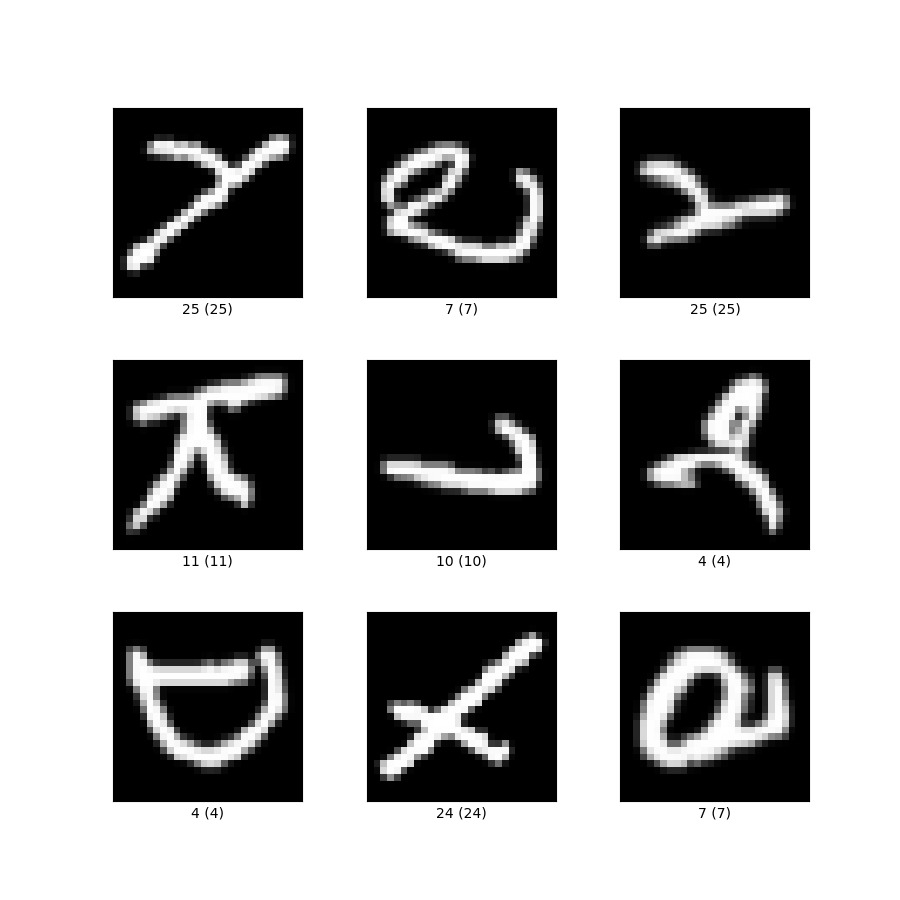
EMNIST is divided into several subsets containing different groupings of characters, including digits, uppercase and lowercase letters, and combinations thereof, allowing researchers and developers to select the subset that best suits their specific needs. These subsets include, for example, EMNIST ByClass, which groups all digits and letters into a single mix of 62 classes, and EMNIST ByMerge, which treats similar letter variants as a single class, reducing the total number of classes and potentially simplifying the classification problem.
Importing EMNIST
To install the EMNIST Python package along with its dependencies, execute the following command:
pip install emnistThe dataset itself is automatically downloaded and cached when needed. To pre-download the data and avoid delay later during program execution, run the following command after installation:
python -c "import emnist; emnist.ensure_cached_data()"Alternatively, if you have already downloaded the original dataset in IDX format from the EMNIST website, copy or move it to /.cache/emnist/, where is your home folder, and rename it from gzip.zip to emnist.zip. The package will use the existing file instead of downloading it again.
Using EMNIST:
The usage of the EMNIST Python package is designed to be very straightforward.
To get a listing of the available subsets:
from emnist import list_datasets
list_datasets()
This will return a list of available subsets such as ['balanced', 'byclass', 'bymerge', 'digits', 'letters', 'mnist']. (Refer to the EMNIST website for details on each of these subsets.)
To load the training samples for the 'digits' subset:
from emnist import extract_training_samples
images, labels = extract_training_samples('digits')
print(images.shape)  # Output: (240000, 28, 28)
print(labels.shape)  # Output: (240000,)
To load the test samples for the 'digits' subset:
from emnist import extract_test_samples
images, labels = extract_test_samples('digits')
print(images.shape)  # Output: (40000, 28, 28)
print(labels.shape)  # Output: (40000,)
The data is extracted directly from the downloaded compressed file to minimize disk usage, and returned as standard numpy arrays.
In our case, we will use the 'balanced' subset, designed to provide a balanced number of examples for each class of characters, including both digits and letters, thus facilitating the training of classification models that require a balance between classes to improve their performance. To load the training or test samples for the 'balanced' subset, simply replace 'digits' with 'balanced' in the extract_training_samples and extract_test_samples commands respectively:
from emnist import extract_training_samples, extract_test_samples
images, labels = extract_training_samples('balanced')
images, labels = extract_test_samples('balanced')
This approach ensures access to a diverse and balanced dataset, optimizing the training and validation process of your classification model.
Development
Model Creation and Training:
import tensorflow as tf
import pandas as pd
import matplotlib.pyplot as plt
import random
import numpy as np
from emnist import extract_training_samples, extract_test_samples

x_train, y_train = extract_training_samples('balanced')
x_test, y_test = extract_test_samples('balanced')
After loading the training and test samples, the next step is to normalize the input data by dividing by 255, converting pixel values from 0-255 to a range of 0-1, facilitating the neural network's learning process.
x_train, x_test = x_train / 255, x_test / 255The class-mapping dictionary is essential for interpreting the model outputs. Since the model predicts numerical classes corresponding to alphanumeric characters, this dictionary maps the numerical indices (dictionary keys) to their respective characters (dictionary values). This mapping is crucial for translating the model's numerical predictions, ranging from 0 to 46, into a human-readable representation, such as digits and letters. For example, a prediction result of 0 would translate to the character '0', while a result of 10 would translate to the letter 'A'. This decoding step is vital for interpreting the results in practical model applications, such as recognizing characters in vehicle license plate images.
class_mapping = {
  0: '0', 1: '1', 2: '2', 3: '3', 4: '4', 5: '5', 6: '6', 7: '7', 8: '8', 9: '9',
  10: 'A', 11: 'B', 12: 'C', 13: 'D', 14: 'E', 15: 'F', 16: 'G', 17: 'H', 18: 'I', 19: 'J',
  20: 'K', 21: 'L', 22: 'M', 23: 'N', 24: 'O', 25: 'P', 26: 'Q', 27: 'R', 28: 'S', 29: 'T',
  30: 'U', 31: 'V', 32: 'W', 33: 'X', 34: 'Y', 35: 'Z', 36: 'a', 37: 'b', 38: 'd', 39: 'e',
  40: 'f', 41: 'g', 42: 'h', 43: 'n', 44: 'q', 45: 'r', 46: 't'
}
The model is defined using TensorFlow's Sequential API, allowing for a clear and sequential construction of the network layers. It consists of a flatten layer that transforms the 28x28 pixel input images into linear vectors, followed by several dense layers with ReLU activation and dropout layers to reduce overfitting. The final layer is a dense layer with 47 units and softmax activation, corresponding to the number of classes in the "balanced" subset, predicting the probability of each class.
model = tf.keras.models.Sequential([
  tf.keras.layers.Flatten(input_shape=(28, 28)),
  tf.keras.layers.Dense(256, activation='relu'),
  tf.keras.layers.Dropout(0.3),
  tf.keras.layers.Dense(256, activation='relu'),
  tf.keras.layers.Dropout(0.3),
  tf.keras.layers.Dense(128, activation='relu'),
  tf.keras.layers.Dense(64, activation='relu'),
  tf.keras.layers.Dense(47, activation='softmax')
])
The model is compiled with the Adam optimizer and sparse categorical crossentropy as the loss function, a common choice for multi-class classification problems. Training is done by calling the fit method of the model, passing the training and test datasets, and specifying the number of epochs. During training, TensorFlow updates the network weights to minimize the loss function.
model.compile(optimizer='adam', loss='sparse_categorical_crossentropy', metrics=['accuracy'])
history_model = model.fit(x_train, y_train, epochs=20, validation_data=(x_test, y_test))
After training, the model is evaluated on the test set to obtain the final loss and accuracy, providing a quantitative measure of its performance. The training results, specifically the loss over epochs for the training and validation sets, are visualized using Matplotlib, offering a graphical representation of the model's learning progress.
Model Evaluation:
# Evaluate the model
test_loss, test_acc = model.evaluate(x_test, y_test)
print(f"Loss: {test_loss}, Accuracy: {test_acc}")

# Predictions on the test set
y_pred = model.predict(x_test)
y_pred_classes = np.argmax(y_pred, axis=1)

# Manual calculation of precision
true_positives = np.sum((y_test == y_pred_classes) & (y_pred_classes == 1))
predicted_positives = np.sum(y_pred_classes == 1)
precision = true_positives / predicted_positives if predicted_positives > 0 else 0
print(f"Precision: {precision}")
After training the learning model for 20 epochs, we can obtain the following data:
Training Loss and Accuracy: At the end of the last epoch (epoch 20), the model shows a training loss of approximately 0.5272 and a training accuracy of around 82.28%. The training loss is a measure of the model's error on the training data, and the accuracy is the proportion of correct predictions.
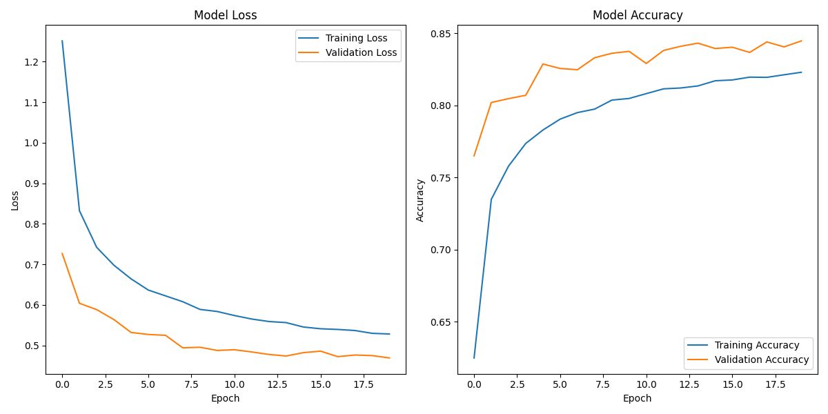
Validation Loss and Accuracy: On the validation data, the model has a similar loss of 0.4926 and an accuracy of 83.85%. The validation data is used to evaluate the model on unseen data during training, so these values are crucial to understand how well the model will generalize to new data.
Test Set Accuracy: After evaluation, the model's accuracy on the test set is approximately 52.78%. This final metric indicates how the model is expected to perform in the real world on completely unseen data.
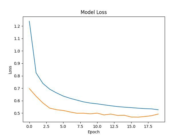
The above graph shows the evolution of the model's loss over the training epochs. Loss is a metric that indicates how well the model is making predictions: the lower the loss, the better the model is predicting. In the graph, the blue line represents the training loss, and the orange line represents the validation or test loss.
We can see that both lines decrease as the number of epochs increases, indicating that the model is learning and improving its performance with each epoch. Ideally, we want the validation loss line to be as low as possible and close to the training loss line, which would suggest that the model is not just memorizing the training data but generalizing well to unseen data.
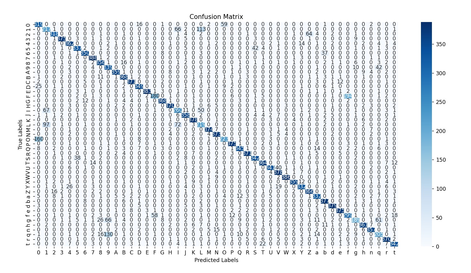
Confusion Matrix: The confusion matrix shows the performance of the character recognition model. The diagonal elements represent correct predictions, where the true label matches the predicted label. Off-diagonal elements indicate misclassifications, where the true label does not match the predicted label. High values along the diagonal suggest the model performs well, while off-diagonal values highlight areas where the model is confused.
Model Export:
Finally, the trained model is saved to the file "license.h5", allowing for later loading and use without the need for retraining. This process encapsulates a typical workflow in deep learning model development, from data preparation to evaluation and use of the trained model.
model.save("license.h5")Vehicle Image Processing:
Image to Process:
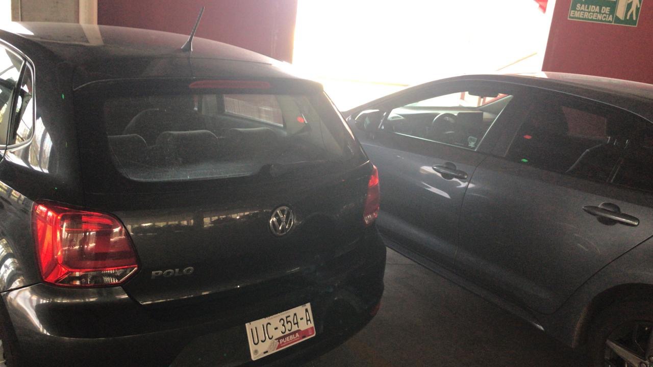
Grid for obtaining coordinates:
To facilitate the image processing workflow, we need to work with coordinates. For this, the following code was generated:
import matplotlib.pyplot as plt
import cv2

# Load the image
image_path = 'nueva_img.jpg'
image = cv2.imread(image_path)

# Convert the image from BGR to RGB for displaying with matplotlib
image_rgb = cv2.cvtColor(image, cv2.COLOR_BGR2RGB)

# Display the image
plt.figure(figsize=(10,5))
plt.imshow(image_rgb)
plt.axis('on')  # to turn on axis numbers
plt.show()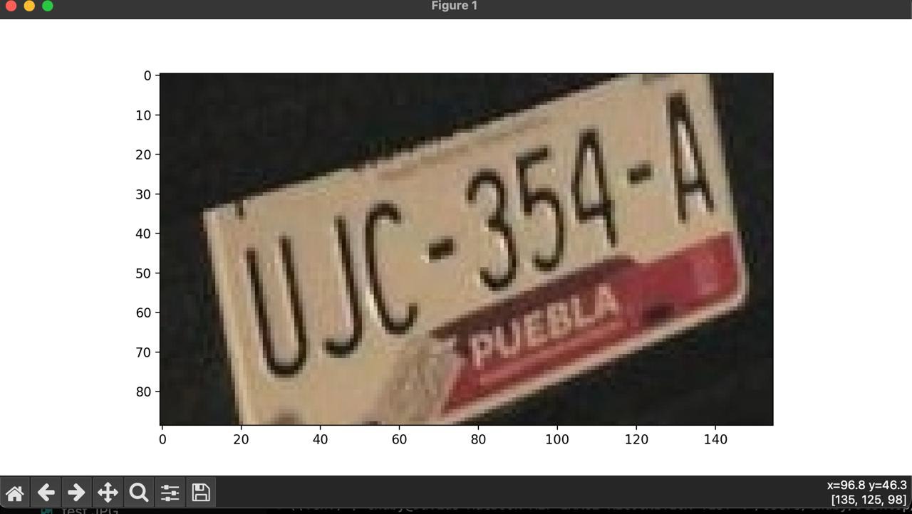
Crop:
The first image processing technique used is cropping to extract only the area where the license plate is located.
import cv2
import numpy as np

image = cv2.imread('test.jpg')
top_left_x = 470
top_left_y = 600
bottom_right_x = 625
bottom_right_y = 689

crop_height = bottom_right_y - top_left_y
crop_width = bottom_right_x - top_left_x

new_image = np.zeros((crop_height, crop_width, 3), dtype=np.uint8)

for i in range(top_left_y, bottom_right_y):
    for j in range(top_left_x, bottom_right_x):
        new_image[i - top_left_y, j - top_left_x] = image[i, j]

cv2.rectangle(image, (top_left_x, top_left_y), (bottom_right_x, bottom_right_y), (0, 255, 0), 3)
cv2.imshow('Original', image)
cv2.imshow('New Image', new_image)
cv2.imwrite('new_image.jpg', new_image)

cv2.waitKey(0)
cv2.destroyAllWindows()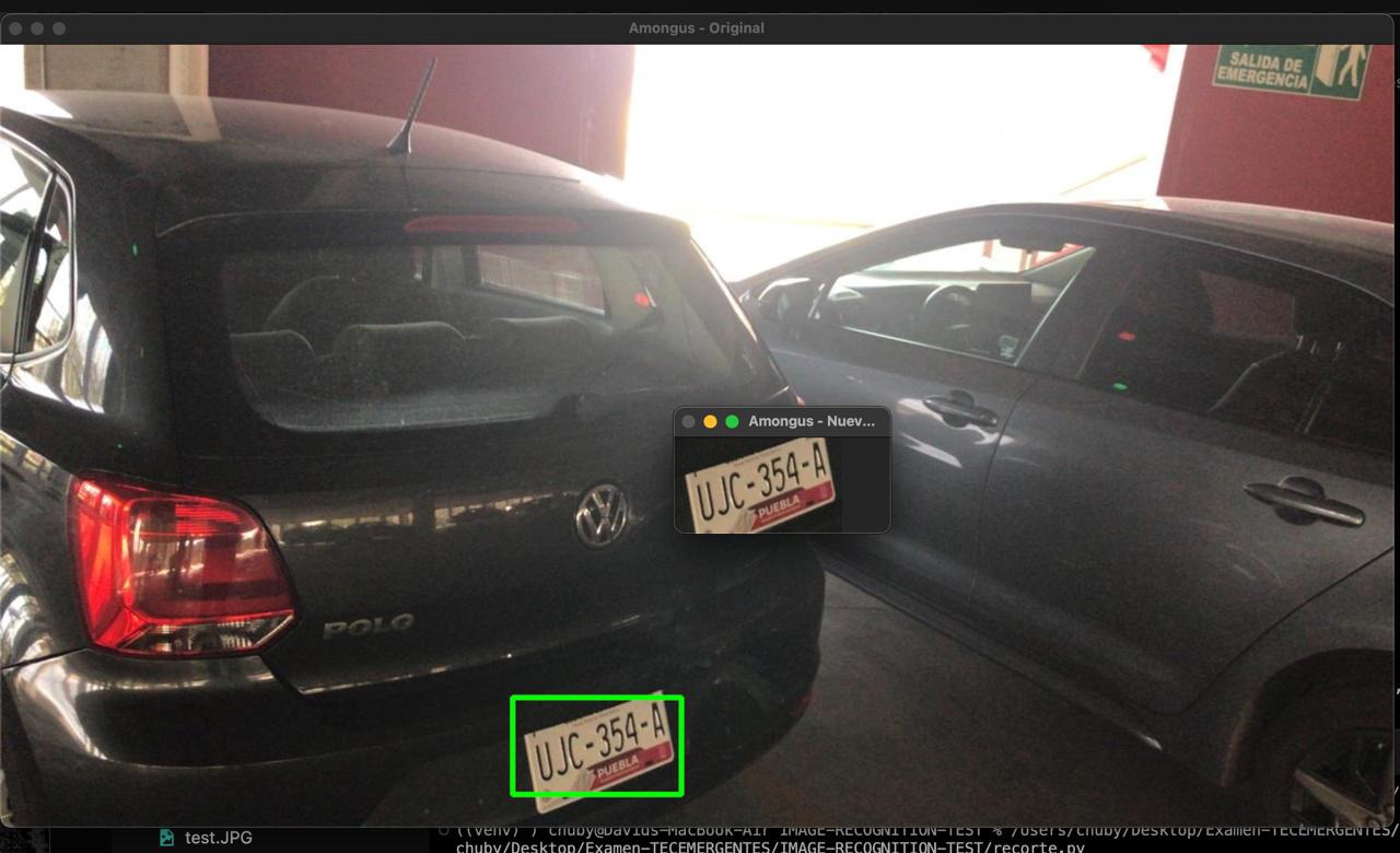
Binarization and Rotation:
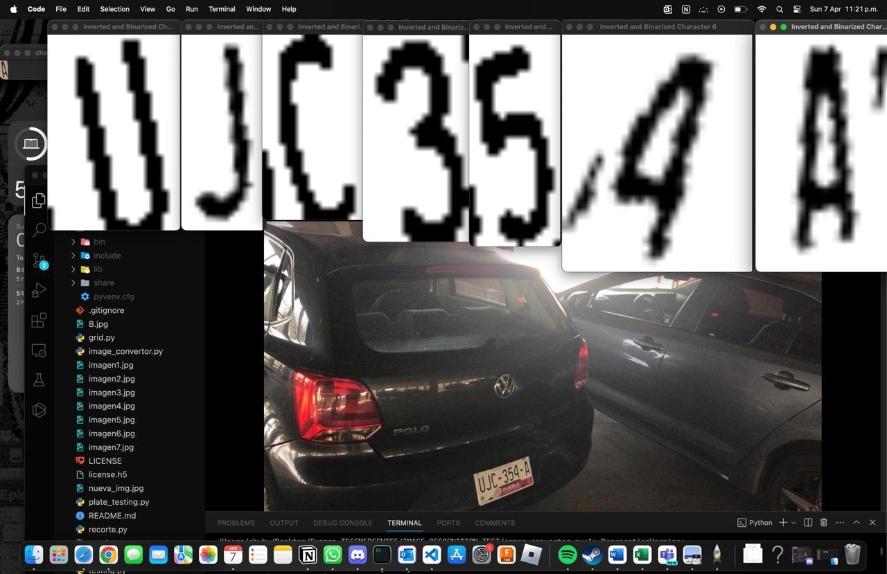
The third block of code contains a set of functions to process the cropped character images. It includes a function for cropping (similar to the first block of code), one for binarizing, and another for rotating the image. Binarization converts the image to grayscale and then to a two-color format, black and white, which facilitates edge detection and character recognition. Rotation is performed with color filling to handle the empty spaces resulting from rotating the image. For each character of the cropped license plate, cropping, color inversion, and binarization are performed, and in some cases, rotation. The processed images are displayed and saved. The code concludes with calls to visualize the images and finally release all window resources created by OpenCV.
import pandas as pd
import numpy as np
import tensorflow as tf
import matplotlib.pyplot as plt
import cv2

def crop(parameters, image):
    top_left_x = parameters['top_left_x']
    top_left_y = parameters['top_left_y']
    bottom_right_x = parameters['bottom_right_x']
    bottom_right_y = parameters['bottom_right_y']
    crop_height = bottom_right_y - top_left_y
    crop_width = bottom_right_x - top_left_x
    new_image = np.zeros((crop_height, crop_width, 3), dtype=np.uint8)
    for i in range(top_left_y, bottom_right_y):
        for j in range(top_left_x, bottom_right_x):
            new_image[i - top_left_y, j - top_left_x] = image[i, j]
    return new_image

def invert_colors_and_binarize(image):
    gray_image = cv2.cvtColor(image, cv2.COLOR_BGR2GRAY)
    _, binary_image = cv2.threshold(gray_image, 127, 255, cv2.THRESH_BINARY)
    return binary_image

def rotate_image_fill(image, angle, fill_color=(255, 255, 255)):
    image_center = tuple(np.array(image.shape[1::-1]) / 2)
    rotation_mat = cv2.getRotationMatrix2D(image_center, angle, 1.0)
    abs_cos = abs(rotation_mat[0, 0])
    abs_sin = abs(rotation_mat[0, 1])
    bound_w = int(image.shape[0] * abs_sin + image.shape[1] * abs_cos)
    bound_h = int(image.shape[0] * abs_cos + image.shape[1] * abs_sin)
    rotation_mat[0, 2] += bound_w / 2 - image_center[0]
    rotation_mat[1, 2] += bound_h / 2 - image_center[1]
    rotated_image = cv2.warpAffine(image, rotation_mat, (bound_w, bound_h), borderValue=fill_color)
    return rotated_image

cropped_plate = cv2.imread('new_image.jpg')
char1 = {'top_left_x': 17, 'top_left_y': 40, 'bottom_right_x': 40, 'bottom_right_y': 74}
char1_cropped = crop(char1, cropped_plate)
cv2.imshow('Char1 - Cropped Image', char1_cropped)

char2 = {'top_left_x': 38, 'top_left_y': 34, 'bottom_right_x': 52, 'bottom_right_y': 74}
char2_cropped = crop(char2, cropped_plate)
cv2.imshow('Char2 - Cropped Image', char2_cropped)

char3 = {'top_left_x': 49, 'top_left_y': 32, 'bottom_right_x': 68, 'bottom_right_y': 64}
char3_cropped = crop(char3, cropped_plate)
cv2.imshow('Char3 - Cropped Image', char3_cropped)

char4 = {'top_left_x': 75, 'top_left_y': 23, 'bottom_right_x': 91, 'bottom_right_y': 54}
char4_cropped = crop(char4, cropped_plate)
cv2.imshow('Char4 - Cropped Image', char4_cropped)

char5 = {'top_left_x': 89, 'top_left_y': 16, 'bottom_right_x': 104, 'bottom_right_y': 51}
char5_cropped = crop(char5, cropped_plate)
cv2.imshow('Char5 - Cropped Image', char5_cropped)

char6 = {'top_left_x': 101, 'top_left_y': 13, 'bottom_right_x': 117, 'bottom_right_y': 45}
char6_cropped = crop(char6, cropped_plate)
cv2.imshow('Char6 - Cropped Image', char6_cropped)

char7 = {'top_left_x': 125, 'top_left_y': 3, 'bottom_right_x': 141, 'bottom_right_y': 40}
char7_cropped = crop(char7, cropped_plate)
cv2.imshow('Char7 - Cropped Image', char7_cropped)

char_images_cropped = [char1_cropped, char2_cropped, char3_cropped, char4_cropped, char5_cropped, char6_cropped, char7_cropped]
char_images_inverted = [invert_colors_and_binarize(img) for img in char_images_cropped]
cv2.imshow('Inverted and Binarized Character 1', char_images_inverted[0])
cv2.imwrite('image1.jpg', char_images_inverted[0])

char2_rotated = rotate_image_fill(char_images_inverted[1], -5, fill_color=(255, 255, 255))
cv2.imshow('Inverted and Binarized Character 2', char2_rotated)
cv2.imwrite('image2.jpg', char2_rotated)

cv2.imshow('Inverted and Binarized Character 3', char_images_inverted[2])
cv2.imwrite('image3.jpg', char_images_inverted[2])

cv2.imshow('Inverted and Binarized Character 4', char_images_inverted[3])
cv2.imwrite('image4.jpg', char_images_inverted[3])

cv2.imshow('Inverted and Binarized Character 5', char_images_inverted[4])
cv2.imwrite('image5.jpg', char_images_inverted[4])

char6_rotated = rotate_image_fill(char_images_inverted[5], -25, fill_color=(255, 255, 255))
char7_rotated = rotate_image_fill(char_images_inverted[6], -10, fill_color=(255, 255, 255))
cv2.imshow('Inverted and Binarized Character 6', char6_rotated)
cv2.imwrite('image6.jpg', char6_rotated)

cv2.imshow('Inverted and Binarized Character 7', char7_rotated)
cv2.imwrite('image7.jpg', char7_rotated)

cv2.waitKey(0)
cv2.destroyAllWindows()
Note that in this format, the letters appear in black and the background in white because when sent to the model, these colors will be inverted and formatted like those in the EMNIST dataset.
Obtaining the Plates:
import tensorflow as tf
import numpy as np
from PIL import Image
import matplotlib.pyplot as plt

# Load the pre-trained model
model = tf.keras.models.load_model('license.h5')

# Class mapping remains the same
class_mapping = {
  0: '0', 1: '1', 2: '2', 3: '3', 4: '4', 5: '5', 6: '6', 7: '7', 8: '8', 9: '9',
  10: 'A', 11: 'B', 12: 'C', 13: 'D', 14: 'E', 15: 'F', 16: 'G', 17: 'H', 18: 'I', 19: 'J',
  20: 'K', 21: 'L', 22: 'M', 23: 'N', 24: 'O', 25: 'P', 26: 'Q', 27: 'R', 28: 'S', 29: 'T',
  30: 'U', 31: 'V', 32: 'W', 33: 'X', 34: 'Y', 35: 'Z', 36: 'a', 37: 'b', 38: 'd', 39: 'e',
  40: 'f', 41: 'g', 42: 'h', 43: 'n', 44: 'q', 45: 'r', 46: 't'
}

predicted_labels = []

# Loop through image files
for i in range(1, 8):  # For image1.jpg to image7.jpg
    img_path = f'image{i}.jpg'
    img = Image.open(img_path)
    img = img.convert('L')  # Convert to grayscale
    img = img.resize((28, 28))  # Resize to match model input
    img = Image.fromarray(255 - np.array(img))  # Invert colors
    img = np.array(img)
    img = img / 255.0  # Normalize
    img = img.reshape(1, 28, 28)  # Reshape for the model

    prediction = model.predict(img)
    label_pred = class_mapping[np.argmax(prediction)]
    predicted_labels.append(label_pred)

    # Optionally display each image with its prediction
    plt.imshow(img[0], cmap='binary_r')
    plt.title(f"Prediction for image{i}.jpg: {label_pred}")
    plt.show()

# Print out values gathered from each prediction
for i, label in enumerate(predicted_labels, start=1):
    print(f"Prediction for image{i}.jpg: {label}")

# Concatenate all labels into a single line
full_prediction = ''.join(predicted_labels)
print(f"Full sequence: {full_prediction}")
This code snippet describes the final phase of the character recognition project, where a pre-trained model is used to predict and analyze individual characters extracted from vehicle license plates. The code covers loading the model to presenting the results.
It starts with loading the trained model named license.h5 using TensorFlow, a deep learning library. This model has already been trained on character images and is ready to make predictions on new data.
The class mapping is a dictionary that maps the model's numerical output to the corresponding alphanumeric characters, allowing for the interpretation of the model's predictions in understandable terms.
The for loop iterates over the image file names from image1.jpg to image7.jpg, which represent each unique character of the plate. Each image is processed through the following steps:
- Convert to grayscale.
- Resize to 28x28 pixels to match the model's expected input.
- Invert the colors, as the model was likely trained with images having light backgrounds and dark characters.
- Normalize the pixels to a range of 0 to 1 to match how the model was trained.
- Reshape the image to the appropriate format expected by the model.
After processing each image, it is fed into the model to get a prediction. The model returns the probability of each class, and the class label with the highest probability is selected as the final prediction for that image.
Analysis and Results
Visualization and Presentation of Results:
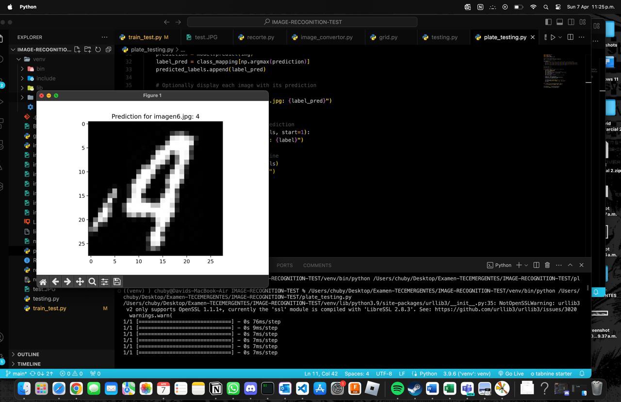
Each image is displayed along with its prediction using Matplotlib for visual inspection. This allows verifying if the prediction makes sense with what is seen in the image. Then, the predicted labels for each image are printed to the console.
Finally, all predicted labels are concatenated into a single string, representing the complete sequence of characters recognized in the vehicle's license plate. This string is crucial for understanding the final result of the character recognition process and has practical applications, such as in automated toll systems or traffic law enforcement.

In the context of analysis and results, this code symbolizes the bridge between data processing and obtaining actionable insights. It illustrates how a trained model can be deployed to obtain verifiable results and how individual results can be combined to obtain a broader conclusion, in this case, the complete identification of a vehicle's license plate.
Conclusion
In conclusion, the project has successfully implemented a robust and efficient character recognition workflow for vehicle license plate identification. Using the EMNIST library for preprocessing and TensorFlow for model construction and training, it has effectively translated the inherent complexity of license plate images into clear and useful predictions. The trained model has demonstrated its ability to accurately predict alphanumeric characters from real images, as evidenced by the tests conducted and the results obtained.
The analysis phase has shown that the images, once processed through the normalization, binarization, and rotation steps as needed, have been adequately interpreted by the model, assigning each a corresponding character with a high degree of confidence. Despite observing a disparity between the model's accuracy on the training and test sets, the tests highlighted the importance of data selection and preparation for the model's performance in uncontrolled environments.
Finally, this modular approach and the techniques used have demonstrated not only the project's viability for specific applications but also its potential scalability and adaptability to different contexts where automatic text recognition is necessary. With possibilities for improvement in accuracy and model generalization, the project establishes a solid foundation for future iterations and developments that can further address the variations and challenges present in real-world text recognition.
The Files:
Below you can find the download links for all of the files from this week.
