Individual Assigment
Design and produce something with a digital process (incorporating computer-aided design and manufacturing) not covered in another assignment, documenting the requirements that your assignment meets, and including everything necessary to reproduce
For this week’s assignment, I decided to focus on a digital process relevant to my final project: developing an object detection and classification application. This task involves working with images, which is a crucial final project.
This assignment is not covered in previous weeks and includes the use of computer-aided design and digital manufacturing in the form of image data generation, training, and deployment of a machine learning model. It meets the criteria by incorporating both digital design and programming to create a working system.
I will divide my work in three parts:
- First, image generation,
- Image labeling
- Model training
- Model prediction
- Counting pest
Image Creation
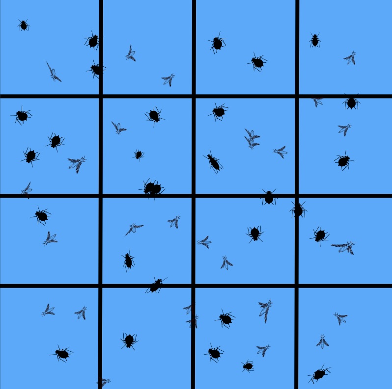
Using Inkscape, I generated an image incorporating two distinct SVG files: one depicting an aphid and the other a thrip, both prevalent greenhouse pests. To simulate commercial pest monitoring tape, I designed a grid layout on a blue surface. Within this grid, I strategically placed the aphid and thrip images, adjusting their positions, scales, and width-to-height ratios to create a varied and representative visual.
Using Inkscape, I generated an image incorporating two distinct SVG files: one depicting an aphid and the other a thrip, both prevalent greenhouse pests. To simulate commercial pest monitoring tape, I designed a grid layout on a blue surface. Within this grid, I placed the aphid and thrip images, downloaded from the internet. I adjusted their positions, scales, and width-to-height ratios to create a varied and representative visual. The final image is displayed below.
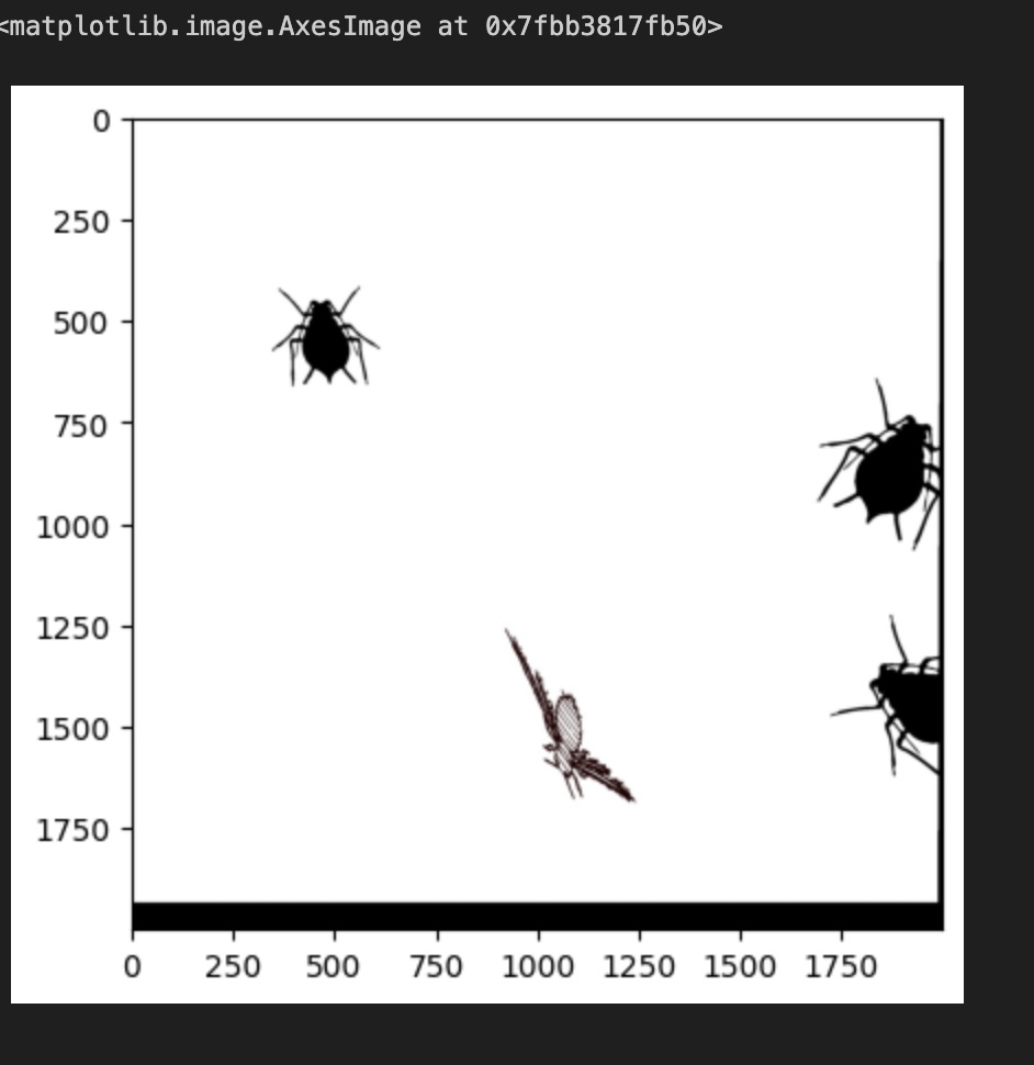
Next, I sliced the image into several sub-pictures, preparing them for data training while reserving a portion for algorithm testing. This process is for demonstration and illustration purposes only. Here is the code.
### Here I import different modules for this task and latter ones.

import matplotlib
import matplotlib.pyplot as plt
import cv2 as cv
import os
from ultralytics import YOLO
import matplotlib.image as img
### Here the image is read and shown
Trap_catch = img.imread('paper_trap_2.jpg')
plt.imshow(Trap_catch)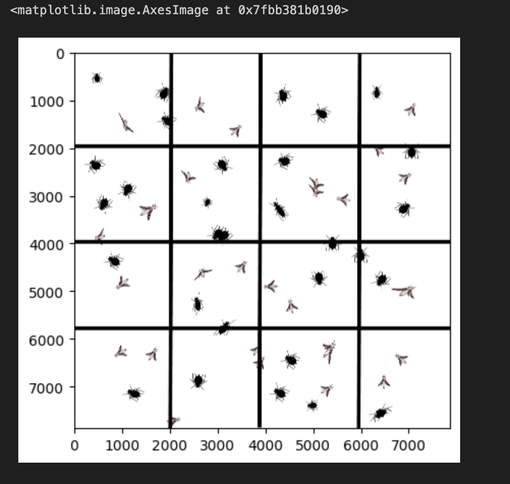 This image contains three matrices, each representing the intensity
values for Red, Green, and Blue (RGB) color channels.
This image contains three matrices, each representing the intensity
values for Red, Green, and Blue (RGB) color channels.
The shape command will output the object’s dimensions as (7874, 7874, 3), representing the x and y values for the three color channels.
Therefore, to slice a specific portion of this grid, we can specify the desired subset of x and y values as shown below.
Here is the code I wrote to slice the grid and display the 16 individual images:
f, imarr = plt.subplots(4,4)
pict=[0, 1960, 3920, 5880, 7840]
counter=0
for i in range(4):
    for ii in range(4):
        TC=Trap_catch[pict[i]:pict[i+1],pict[ii]:pict[ii+1],0:3]
        filename="./raw_images/Grid_"+str(counter)+".jpg"
        matplotlib.image.imsave(filename, TC)
        imarr[i,ii].imshow(TC)
        counter+=1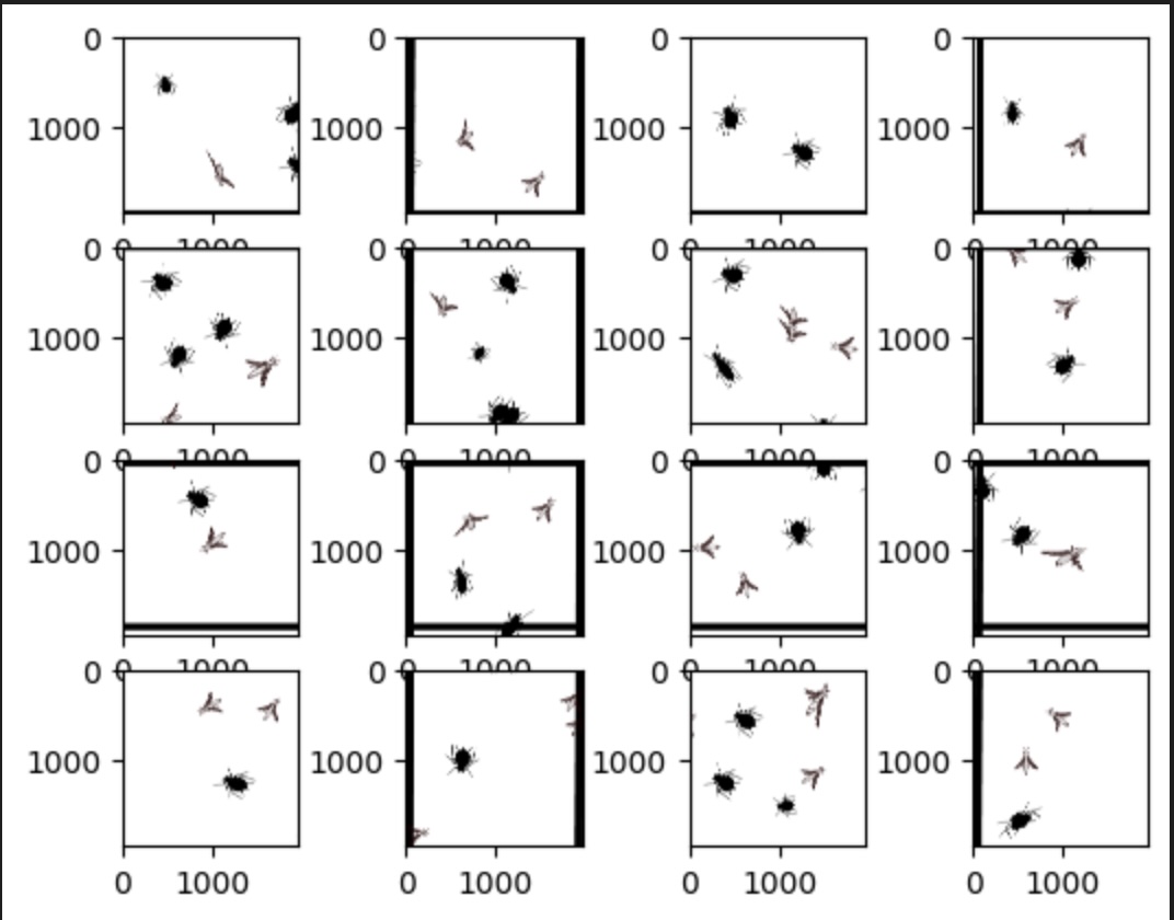
Then divided the image into 10 sub-images for training the model, while reserving 4 sub-images for validation and testing. This setup is intended to demonstrate the core concept, logic and workflow of the approach.
Image Annotation
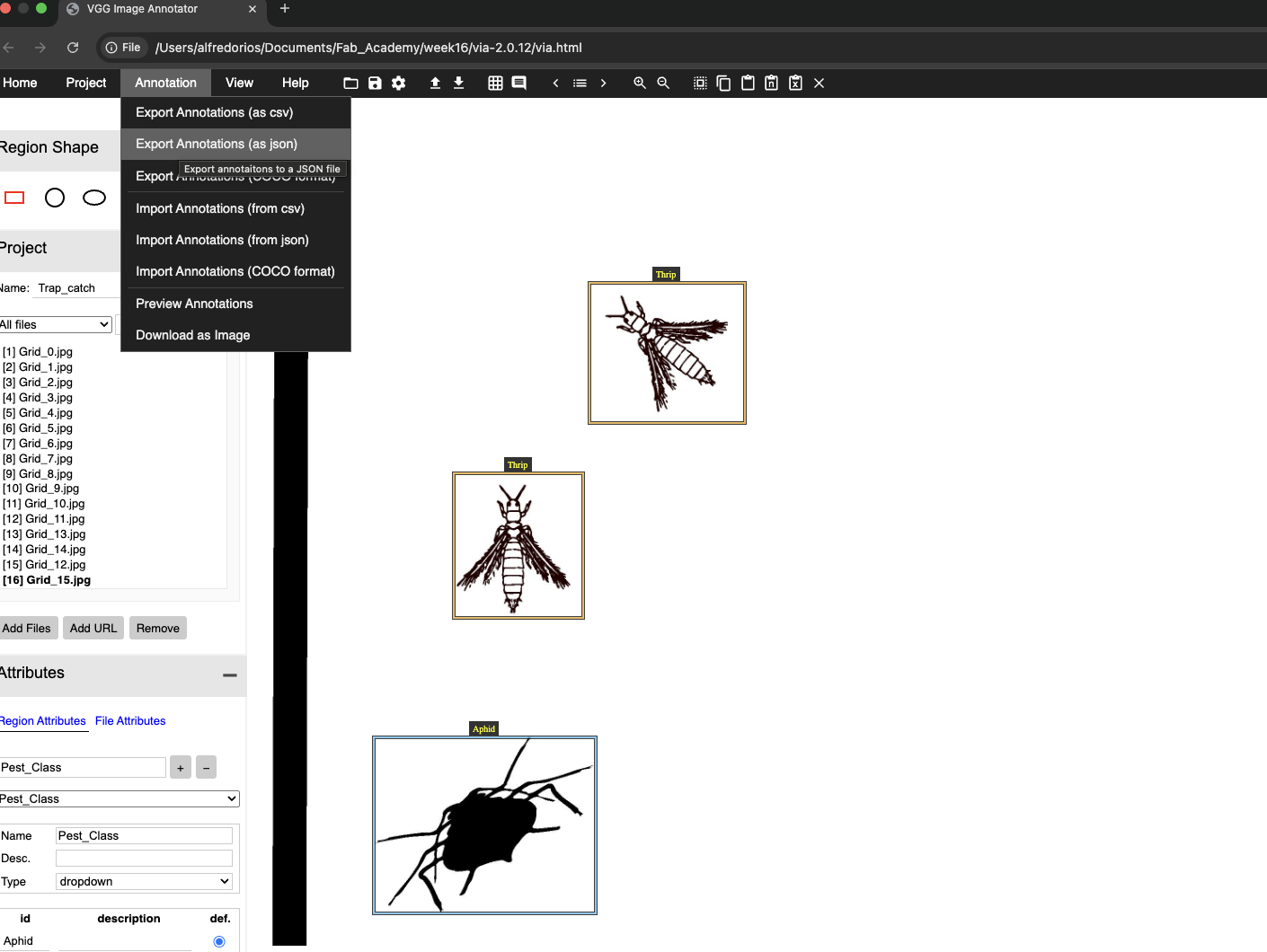
Building on that, I then sought out an open-source annotation tool and discovered the VGG Image Annotator. This tool greatly facilitates the process of annotating objects within images. I also followed a tutorial that explains how the tool is used.
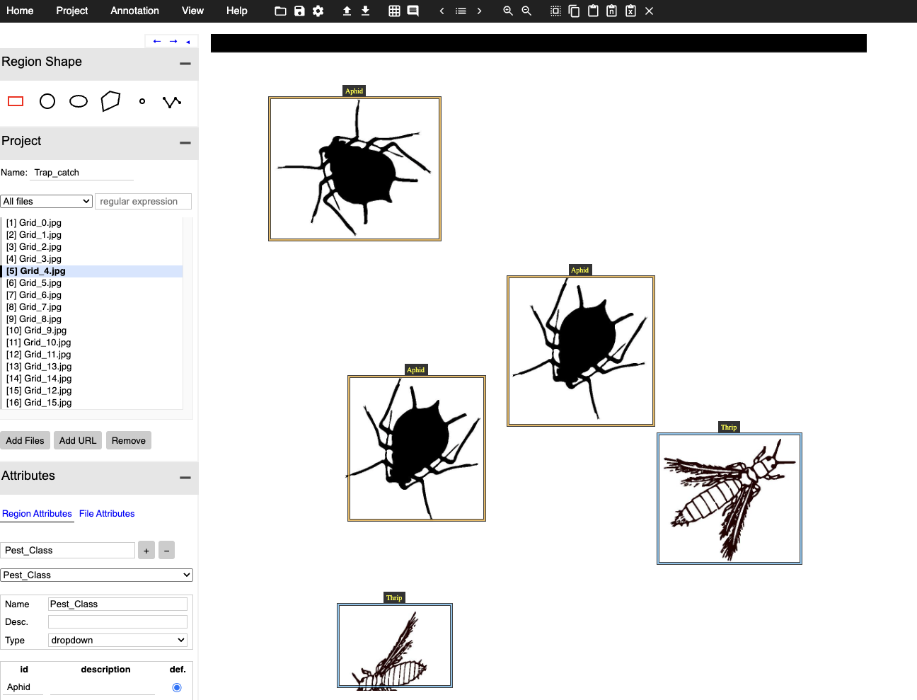
Here is an image of VGG, which is essentially a web-based tool that you can use online or download for offline use.
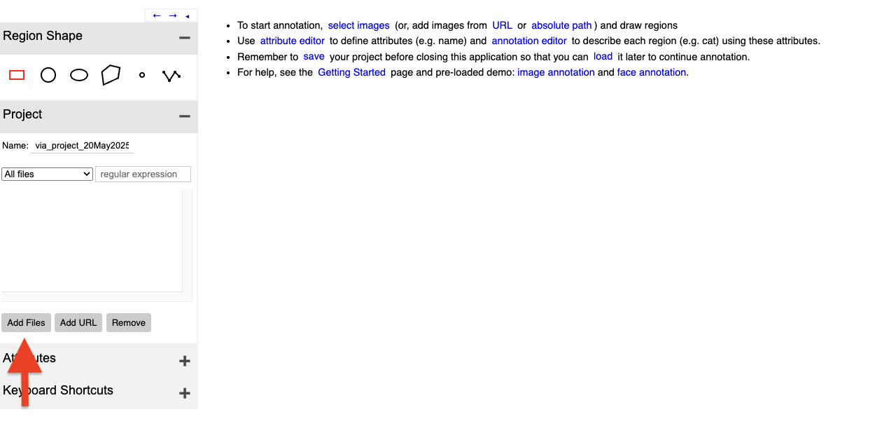
On the webpage, you can add images by clicking the Add button located in the upper-left panel. Here you can see a display of the first image. On the lower left panel you can add attributes that is the attribute you want to detect.
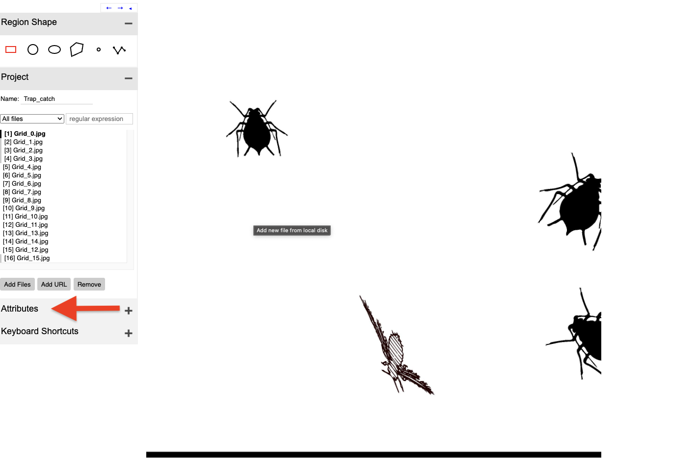
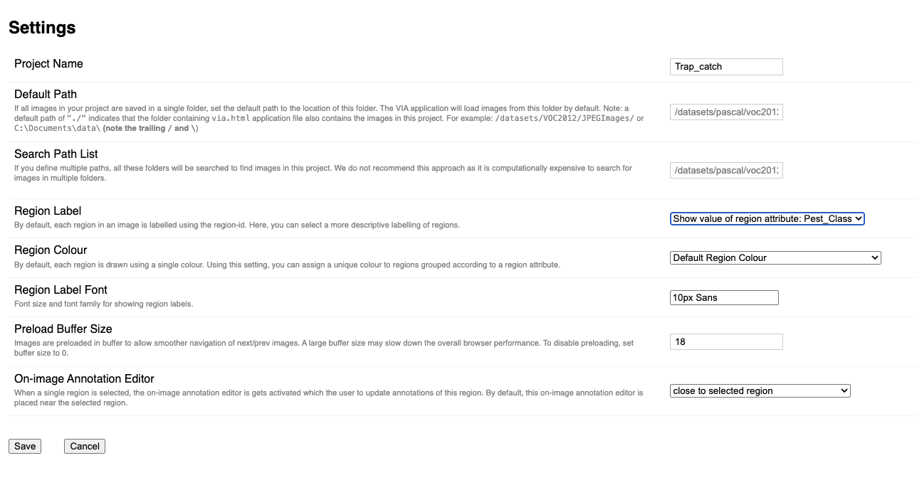
In my case, I added a Pest_Class attribute and used a dropdown widget to allow the user to select the class to which each object belongs.
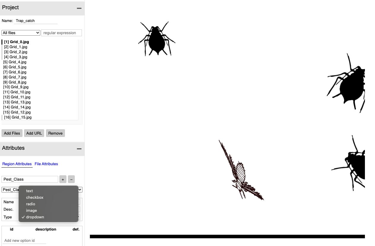
Here, I entered the object classes (aphid and thrip) and used a radio button to set the default class to the most common one.
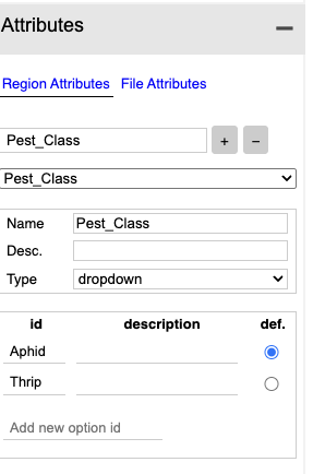
Finally, there is a setting to choose whether the classes should appear as numerical labels or as the category names.
Here, you can see the labeling process in action. The user selects the appropriate category from the dropdown menu that was previously configured.
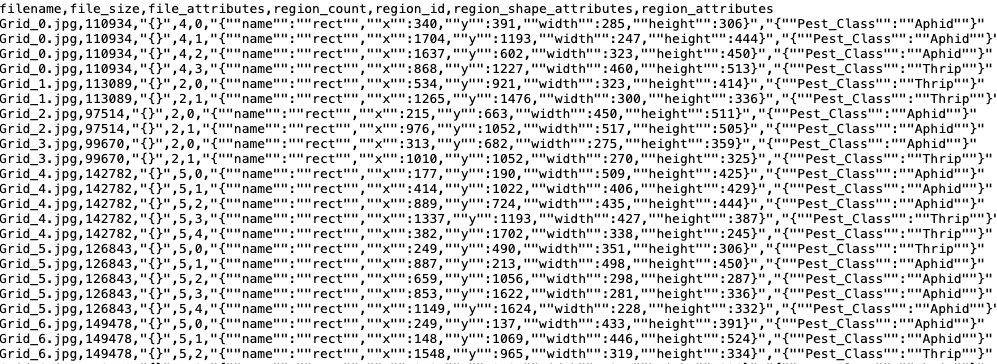
 Below you can see what the
application does. It basically provides the coordinates for the bounding
boxes and the pest class label.
Below you can see what the
application does. It basically provides the coordinates for the bounding
boxes and the pest class label.
 Note that this app allows you
to save your progress as you work. Finally one can export the file in
different formats. I chose json.
Note that this app allows you
to save your progress as you work. Finally one can export the file in
different formats. I chose json.
Yolo Model Implementation
I knew the labeled data needed to be converted to the YOLO format, so I asked ChatGPT to generate code for this conversion. Below is the prompt I used.
what format do I need to export annotated images to Yolo8 …how about if I am using VGG
# === SETTINGS ===
via_json = "/Users/alfredorios/Documents/Fab_Academy/week16/Trap_catch.json"       # Your VIA annotation file
image_dir = "/Users/alfredorios/Documents/Fab_Academy/week16/raw_images"                # Folder containing all 16 images
output_dir = "/Users/alfredorios/Documents/Fab_Academy/week16/Yolo_file_structure"             # Output folder for YOLOv8 structure

# Define class name to ID mapping
class_map = {
    "Aphid": 0,
    "Thrip": 1,
    # Add more as needed
}

# Create YOLOv8 folder structure
splits = ["train", "val", "test"]
for split in splits:
    os.makedirs(f"{output_dir}/images/{split}", exist_ok=True)
    os.makedirs(f"{output_dir}/labels/{split}", exist_ok=True)

# Load VIA JSON
with open(via_json, 'r') as f:
    data = json.load(f)

# Get and shuffle image keys
image_keys = list(data["_via_img_metadata"].keys())
random.shuffle(image_keys)  # Optional: for randomness

# Fixed split
train_keys = image_keys[:10]
val_keys   = image_keys[10:13]
test_keys  = image_keys[13:]

def convert_box(shape, width, height):
    x = shape["x"]
    y = shape["y"]
    w = shape["width"]
    h = shape["height"]
    x_center = (x + w / 2) / width
    y_center = (y + h / 2) / height
    return x_center, y_center, w / width, h / height

def export(split_keys, split_name):
    for key in split_keys:
        file_data = data["_via_img_metadata"][key]
        filename = file_data["filename"]
        regions = file_data["regions"]

        src_path = os.path.join(image_dir, filename)
        dst_img = os.path.join(output_dir, "images", split_name, filename)
        dst_label = os.path.join(output_dir, "labels", split_name, filename.rsplit(".", 1)[0] + ".txt")

        # Copy image
        if not os.path.exists(src_path):
            raise FileNotFoundError(f"Image not found: {src_path}")
        shutil.copy(src_path, dst_img)

        # Get image dimensions
        with Image.open(src_path) as img:
            width, height = img.size

        lines = []
        for region in regions:
            shape = region["shape_attributes"]
            attrs = region["region_attributes"]

            if shape["name"] != "rect":
                continue

            class_name = list(attrs.values())[0] if attrs else "unknown"
            class_id = class_map.get(class_name, -1)
            if class_id == -1:
                print(f"Warning: Unmapped class '{class_name}'")
                continue

            x_c, y_c, w, h = convert_box(shape, width, height)
            lines.append(f"{class_id} {x_c:.6f} {y_c:.6f} {w:.6f} {h:.6f}")

        # Save annotation file
        with open(dst_label, 'w') as out:
            out.write("\n".join(lines))

# Export all splits
export(train_keys, "train")
export(val_keys, "val")
export(test_keys, "test")
Next, I proceeded to implement the YOLO object detection model using the converted data.
### This are the preliminaries
from ultralytics import YOLO
import supervision as sv
bounding_box_annotator=sv.BoundingBoxAnnotator()
label_annotator=sv.LabelAnnotator()
Here, I set up the model architecture and then proceeded to train it.
model = YOLO("yolov8n.pt")

results = model.train(data=os.path.join("/Users/alfredorios/Documents/Fab_Academy/week16/Yolo_file_structure", "data.yaml"), epochs=100)
The arguments specify the path to the data files, the name of the YAML file that defines the dataset structure, and the list of object class names. Additionally, they include the number of training epochs. Below you can find the yaml file used.
path: /Users/alfredorios/Documents/Fab_Academy/week16/Yolo_file_structure
train: images/train
val: images/val
test: images/test

names:
  0: Aphid
  1: Thrip
This is the output from Yolo:
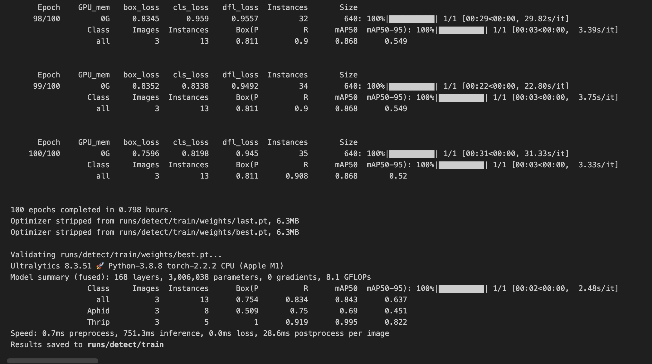
It took about 50 minutes to run the 100 epochs.
The metrics are covered in this link.
Two of which are reproduced below:
- P(Precision): The accuracy of the detected objects, indicating how many detections were correct.
- R(Recall): The ability of the model to identify all instances of objects in the images.
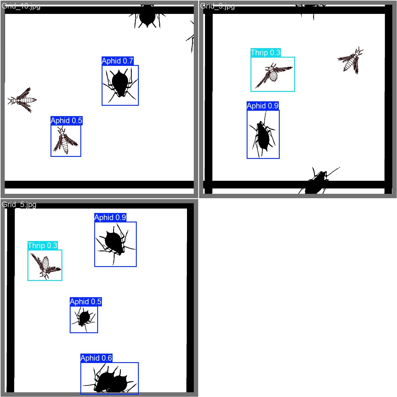
We retrieve the prediction on the validation data set.
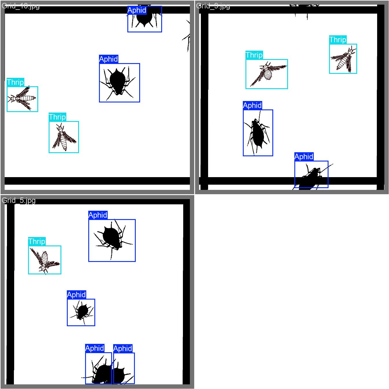
For comparison, here are the labeled images.
To enable a systematic comparison, the confusion matrix below shows how the “real” objects were predicted by the model.
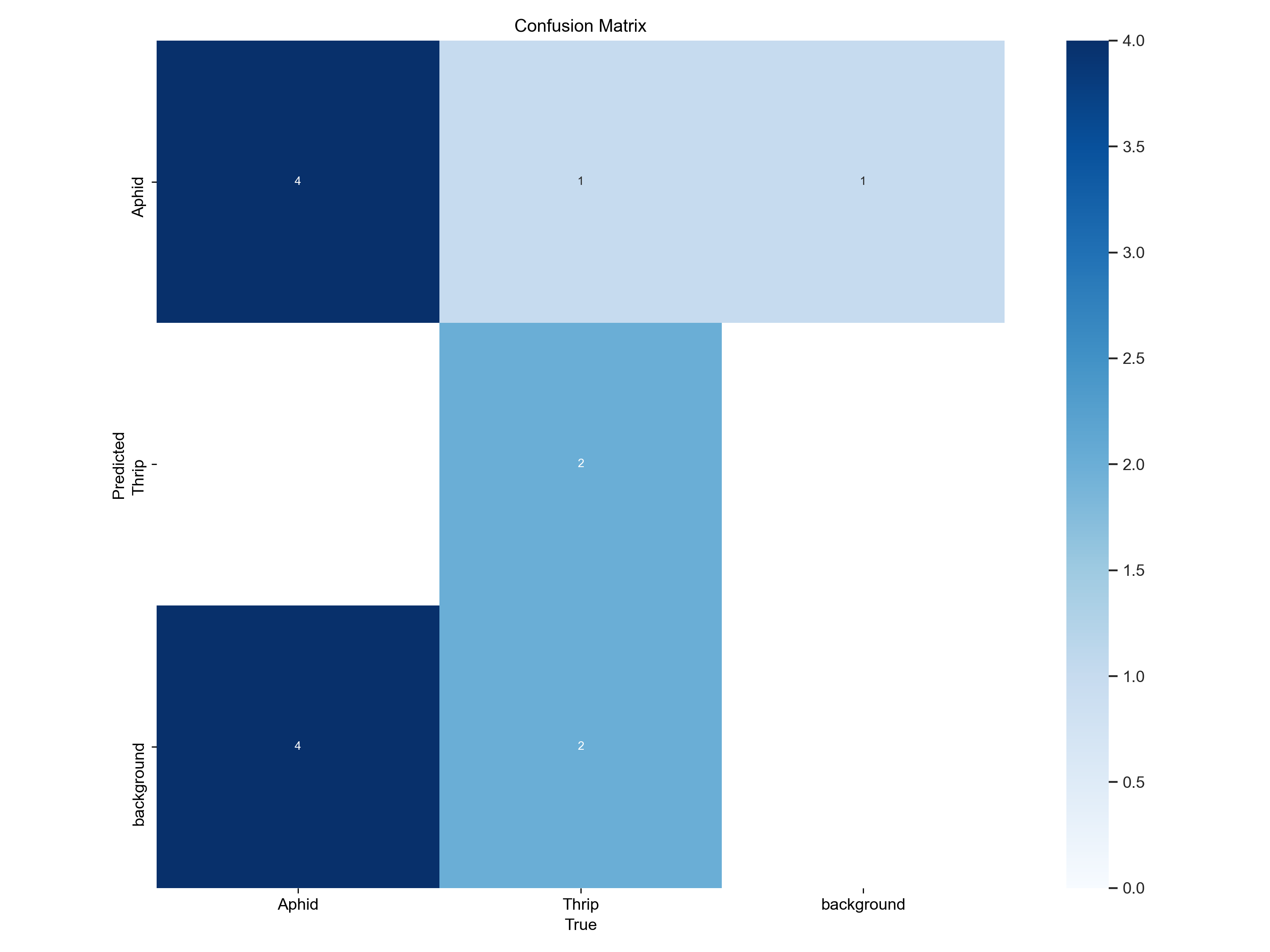 Here for example we can see that 4 aphids were
predicted as aphids, 0 as thrips and four as background.
Here for example we can see that 4 aphids were
predicted as aphids, 0 as thrips and four as background.
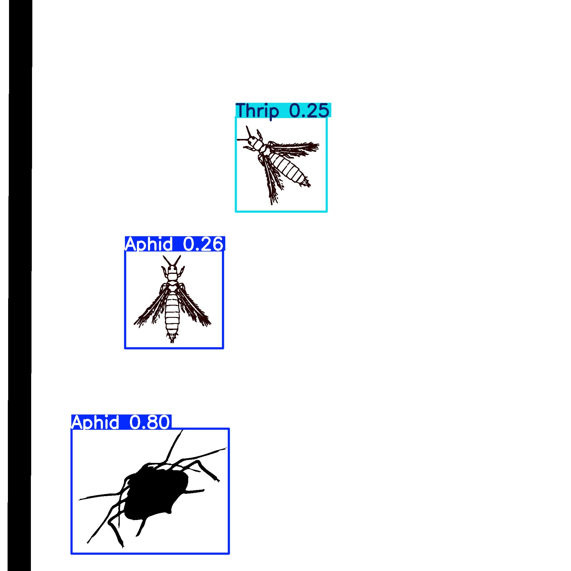
Predictions
Below are the commands to load the model weights and perform predictions.
And here you can point to the directory where to find the images for prediction.
new_prediction=model("/Users/alfredorios/Documents/Fab_Academy/week16/Yolo_file_structure/images/test")Finally, you can display the image with the following command.
Link to development page
Learning outcomes
- Demonstrate workflows used in the chosen process
- Select and apply suitable processes (and materials) to do your assignment.
- Have you answered these questions?
Have you?
- Documented the workflow(s) and process(es) you used
- Explained how your process is not covered on other assignments
- Described problems encountered (if any) and how you fixed them
- Included original design files and source code
- Included ‘hero shot’ of the result